---
title: "Joining Data (Notes)"
format:
html:
toc: true
toc-depth: 2
embed-resources: true
---
```{r include = FALSE}
# This chunk just sets up some styling (eg: default size of our images)
knitr::opts_chunk$set(
collapse = TRUE,
warning = FALSE,
message = FALSE,
fig.height = 2.75,
fig.width = 4.25,
fig.align = 'center')
```
::: {.callout-note title="Learning goals"}
Understand how to *join* different datasets:
- mutating joins: `left_join()`, `inner_join()` and `full_join()`
- filtering joins: `semi_join()`, `anti_join()`
:::
\
\
\
\
::: {.callout-note title="Additional resources"}
Watch:
- [Demonstration of joining data](https://www.youtube.com/watch?v=MJDHRtwZhoM&feature=youtu.be) (Lisa Lendway)
Read:
- [Joings](https://r4ds.hadley.nz/joins) (Wickham, Çetinkaya-Rundel, & Grolemund)
- [Data wrangling on multiple tables](https://mdsr-book.github.io/mdsr2e/ch-join.html) (Baumer, Kaplan, and Horton)
:::
\
\
\
\
## Warm-up
**Where are we? Data preparation**
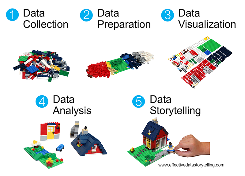
Thus far, we've learned how to:
- `arrange()` our data in a meaningful order
- subset the data to only `filter()` the rows and `select()` the columns of interest
- `mutate()` existing variables and define new variables
- `summarize()` various aspects of a variable, both overall and by group (`group_by()`)
- reshape our data to fit the task at hand (`pivot_longer()`, `pivot_wider()`)
\
\
\
\
**Motivation**
In practice, we often have to collect and combine data from various sources in order to address our research questions. Example:
- What are the best predictors of album sales?\
Combine:
- Spotify data on individual songs (eg: popularity, genre, characteristics)
- sales data on individual songs
- What are the best predictors of flight delays?\
Combine:
- data on individual flights including airline, starting airport, and destination airport
- data on different airlines (eg: ticket prices, reliability, etc)
- data on different airports (eg: location, reliability, etc)
\
\
\
\
**EXAMPLE 1**
Consider the following (made up) data on students and course enrollments:
```{r}
students_1 <- data.frame(
student = c("A", "B", "C", "A"),
class = c("STAT 101", "GEOL 101", "ANTH 101", "GEOL 101")
)
# Check it out
students_1
```
```{r}
enrollments_1 <- data.frame(
class = c("STAT 101", "ART 101", "GEOL 101"),
enrollment = c(18, 17, 24)
)
# Check it out
enrollments_1
```
Imagine someone says to you: "For each student, I want to know the enrollment of each class the student is taking."
Work this out by hand: make a table with three columns: student, class, enrollment.
Here are the two datasets side-by-side:
```
> students_1 > enrollments_1
student class class enrollment
1 A STAT 101 1 STAT 101 18
2 B GEOL 101 2 ART 101 17
3 C ANTH 101 3 GEOL 101 24
4 A GEOL 101
```
**When you are done**: think carefully about how you constructed your table and exactly what you did with the two tables to get the numbers in the enrollment column.
Write a short sentence describing what you did.
\
\
\
\
**Other questions**
Consider the following questions that we might also ask of this type of data. Do they sound like reasonable questions that might be asked?
- "For each student, I want to know the enrollment of each class the student is taking, but I don't care about any student for whom we don't have enrollment data."
- "I want to see this enrollment data for all students -- and I also want to see which courses don't have any of these students enrolled in them."
- "I want to see students and classes for which there's no matching enrollment data."
\
\
\
\
**Joins**
Answering the questions above required you to *combine* or *join* these datasets into one.
**How can we make R do the same thing we did when making our table?**
First, consider the following:
- What variable or **key** do these datasets have in common? Thus by what information can we *match* the observations in these datasets?
- Relative to this key, what info does `students_1` have that `enrollments_1` doesn't?
- Relative to this key, what info does `enrollments_1` have that `students_1` doesn't?
\
\
\
\
**EXAMPLE 2**
There are various ways to join these datasets:
```
> students_1 > enrollments_1
student class class enrollment
1 A STAT 101 1 STAT 101 18
2 B GEOL 101 2 ART 101 17
3 C ANTH 101 3 GEOL 101 24
4 A GEOL 101
```
Let's learn by doing. First, try the `left_join()` function:
```{r}
library(tidyverse)
students_1 %>%
left_join(enrollments_1)
```
- What did this do?
- Which observations from `students_1` (the *left* table) were retained?
- Which observations from `enrollments_1` (the *right* table) were retained?
- What, if anything, would change if we reversed the order of the data tables? Think about it, then try.
```{r}
```
\
\
\
\
**EXAMPLE 3**
Next, explore how our datasets are joined using `inner_join()`:
```
> students_1 > enrollments_1
student class class enrollment
1 A STAT 101 1 STAT 101 18
2 B GEOL 101 2 ART 101 17
3 C ANTH 101 3 GEOL 101 24
4 A GEOL 101
```
```{r}
students_1 %>%
inner_join(enrollments_1)
```
- What did this do?
- Which observations from `students_1` (the *left* table) were retained?
- Which observations from `enrollments_1` (the *right* table) were retained?
- What, if anything, would change if we reversed the order of the data tables? Think about it, then try.
```{r}
```
\
\
\
\
**EXAMPLE 4**
Next, explore how our datasets are joined using `full_join()`:
```
> students_1 > enrollments_1
student class class enrollment
1 A STAT 101 1 STAT 101 18
2 B GEOL 101 2 ART 101 17
3 C ANTH 101 3 GEOL 101 24
4 A GEOL 101
```
```{r}
students_1 %>%
full_join(enrollments_1)
```
- What did this do?
- Which observations from `students_1` (the *left* table) were retained?
- Which observations from `enrollments_1` (the *right* table) were retained?
- What, if anything, would change if we reversed the order of the data tables? Think about it, then try.
```{r}
```
\
\
\
\
**Mutating joins: left, inner, full**
Mutating joins add new variables (columns) to the left data table from matching observations in the right table:
`left_data %>% mutating_join(right_data)`
The most common mutating joins are:
- `left_join()`\
Keeps *all* observations from the left, but discards any observations in the right that do not have a match in the left.[^11-joining-data-1]
- `inner_join()`\
Keeps *only* the observations from the left with a match in the right.
- `full_join()`\
Keeps *all* observations from the left *and* the right. (This is less common than `left_join()` and `inner_join()`).
[^11-joining-data-1]: There is also a `right_join()` that adds variables in the reverse direction from the left table to the right table, but we do not really need it as we can always switch the roles of the two tables.︎
NOTE: When an observation in the left table has *multiple* matches in the right table, these mutating joins produce a *separate* observation in the new table for each match.
\
\
\
\
**EXAMPLE 5**
*Mutating* joins *combine* information, thus increase the number of columns in a dataset (like `mutate()`). *Filtering* joins keep only certain observations in one dataset (like `filter()`), not based on rules related to any variables in the dataset, but on the observations that exist in another dataset. This is useful when we merely care about the membership or non-membership of an observation in the other dataset, not the raw data itself.
In our example data, suppose `enrollments_1` only included courses being taught in the Theater building:
```
> students_1 > enrollments_1
student class class enrollment
1 A STAT 101 1 STAT 101 18
2 B GEOL 101 2 ART 101 17
3 C ANTH 101 3 GEOL 101 24
4 A GEOL 101
```
```{r}
students_1 %>%
semi_join(enrollments_1)
```
- What did this do? What info would it give us?
- How does `semi_join()` differ from `inner_join()`?
- What, if anything, would change if we reversed the order of the data tables? Think about it, then try.
```{r}
```
\
\
\
\
**EXAMPLE 6**
Let's try another filtering join for our example data:
```
> students_1 > enrollments_1
student class class enrollment
1 A STAT 101 1 STAT 101 18
2 B GEOL 101 2 ART 101 17
3 C ANTH 101 3 GEOL 101 24
4 A GEOL 101
```
```{r}
students_1 %>%
anti_join(enrollments_1)
```
- What did this do? What info would it give us?
- What, if anything, would change if we reversed the order of the data tables? Think about it, then try.
```{r}
```
\
\
\
\
**Filtering joins: semi, anti**
Filtering joins keep specific observations from the left table based on whether they match an observation in the right table.
- `semi_join()`\
Discards any observations in the left table that *do not* have a match in the right table. If there are multiple matches of right cases to a left case, it keeps just one copy of the left case.
- `anti_join()`\
Discards any observations in the left table that *do* have a match in the right table.
\
\
\
\
\
\
**A SUMMARY OF ALL OF OUR JOINS**
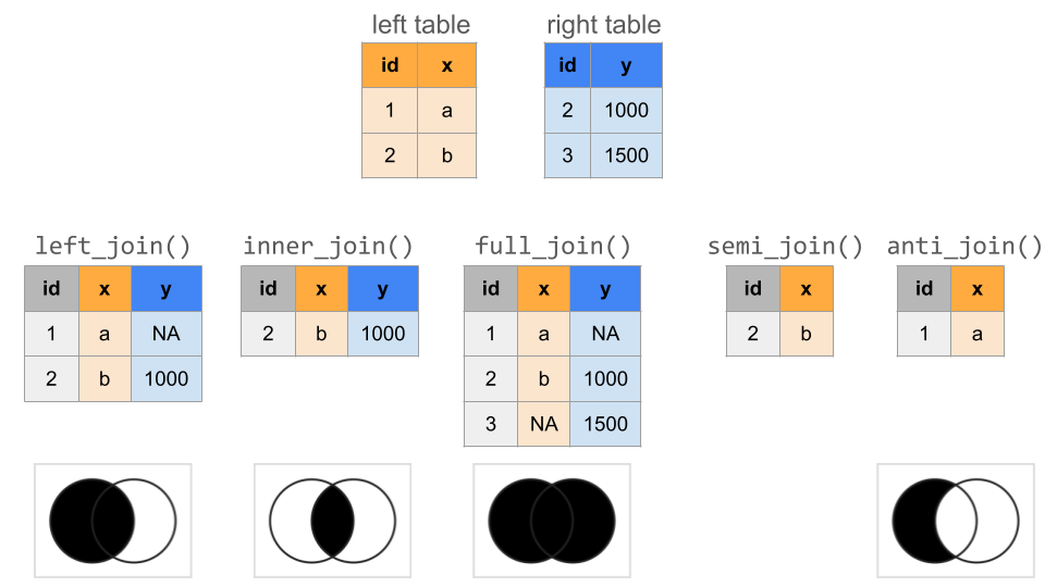
Useful RStudio cheat sheets:
- Data transformation cheat sheet: [HTML](https://rstudio.github.io/cheatsheets/html/data-transformation.html), [PDF](https://rstudio.github.io/cheatsheets/data-transformation.pdf)
- Includes our 6 wrangling verbs and joins
- Data tidying cheat sheet: [HTML](https://rstudio.github.io/cheatsheets/html/tidyr.html), [PDF](https://rstudio.github.io/cheatsheets/tidyr.pdf)
- Includes `pivot_longer()` and `pivot_wider()` for reshaping our data
\
\
\
\
\
## Exercises
**Goals**
Now that we understand the basics, let's:
- Explore some subtleties of the `join()` functions.
- Apply the `join()` functions to bigger datasets.
\
\
**Directions**
- Work together and stay in relative sync! You should not be on Exercise 10 if the group is on Exercise 2.
- Help create an environment where everyone feels comfortable asking questions and sharing ideas. Again, this is hard to do if you're on Exercise 10 while the group is on Exercise 2.
- When *you* have questions, speak up. First discuss your question with the group. If the group cannot identify a solution, ask me!
\
\
### Exercise 1: Where are my keys? {.unnumbered}
#### Part a {.unnumbered}
Define two new datasets, with different students and courses:
```{r}
students_2 <- data.frame(
student = c("D", "E", "F"),
class = c("COMP 101", "BIOL 101", "POLI 101")
)
# Check it out
students_2
enrollments_2 <- data.frame(
course = c("ART 101", "BIOL 101", "COMP 101"),
enrollment = c(18, 20, 19)
)
# Check it out
enrollments_2
```
To connect the course enrollments to the students' courses, try do a `left_join()`. You get an error! Identify the problem by reviewing the error message and the datasets we're trying to join.
```{r eval = FALSE}
# eval = FALSE: don't evaluate this chunk when knitting. it produces an error.
students_2 %>%
left_join(enrollments_2)
```
#### Part b {.unnumbered}
The problem is that course name, the **key** or variable that links these two datasets, is labeled differently: `class` in the `students_2` data and `course` in the `enrollments_2` data. Thus we have to specify these keys in our code:
```{r}
students_2 %>%
left_join(enrollments_2, by = c("class" = "course"))
```
```{r eval = FALSE}
# The order of the keys is important:
# by = c("left data key" = "right data key")
# The order is mixed up here, thus we get an error:
students_2 %>%
left_join(enrollments_2, by = c("course" = "class"))
```
#### Part c {.unnumbered}
Define another set of fake data which adds grade information:
```{r}
# Add student grades in each course
students_3 <- data.frame(
student = c("Y", "Y", "Z", "Z"),
class = c("COMP 101", "BIOL 101", "POLI 101", "COMP 101"),
grade = c("B", "S", "C", "A")
)
# Check it out
students_3
# Add average grades in each course
enrollments_3 <- data.frame(
class = c("ART 101", "BIOL 101","COMP 101"),
grade = c("B", "A", "A-"),
enrollment = c(20, 18, 19)
)
# Check it out
enrollments_3
```
Try doing a `left_join()` to link the students' classes to their enrollment info. Did this work? Try and figure out the culprit by examining the output.
```{r}
students_3 %>%
left_join(enrollments_3)
```
#### Part d {.unnumbered}
The issue here is that our datasets have *2* column names in common: `class` and `grade`. BUT `grade` is measuring 2 different things here: individual student grades in `students_3` and average student grades in `enrollments_3`. Thus it doesn't make sense to try to join the datasets with respect to this variable. We can again solve this by specifying that we want to join the datasets using the `class` variable or *key*. What are `grade.x` and `grade.y`?
```{r}
students_3 %>%
left_join(enrollments_3, by = c("class" = "class"))
```
\
\
\
\
### Exercise 2: More small practice {.unnumbered}
Before applying these ideas to bigger datasets, let's practice identifying which join is appropriate in different scenarios. Define the following fake data on `voters` (people who *have* voted) and `contact` info for voting age adults (people who *could* vote):
```{r}
# People who have voted
voters <- data.frame(
id = c("A", "D", "E", "F", "G"),
times_voted = c(2, 4, 17, 6, 20)
)
voters
# Contact info for voting age adults
contact <- data.frame(
name = c("A", "B", "C", "D"),
address = c("summit", "grand", "snelling", "fairview"),
age = c(24, 89, 43, 38)
)
contact
```
Use the appropriate join for each prompt below. In each case, think before you type:
- What dataset goes on the left?
- What do you want the resulting dataset to look like? How many rows and columns will it have?
```{r}
# 1. We want contact info for people who HAVEN'T voted
# 2. We want contact info for people who HAVE voted
# 3. We want any data available on each person
# 4. When possible, we want to add contact info to the voting roster
```
\
\
\
\
### Exercise 3: Bigger datasets {.unnumbered}
Let's apply these ideas to some bigger datasets. In `grades`, each row is a student-class pair with information on:
- `sid` = student ID
- `sessionID` = an identifier of the class section
- `grade` = student's grade
```{r echo = FALSE}
# Get rid of some duplicate rows!
grades <- read.csv("https://mac-stat.github.io/data/grades.csv") %>%
distinct(sid, sessionID, .keep_all = TRUE)
# head(grades)
```
In `courses`, each row corresponds to a class section with information on:
- `sessionID` = an identifier of the class section
- `dept` = department
- `level` = course level (eg: 100)
- `sem` = semester
- `enroll` = enrollment (number of students)
- `iid` = instructor ID
```{r echo = FALSE}
courses <- read.csv("https://mac-stat.github.io/data/courses.csv")
# head(courses)
```
Use R code to take a quick glance at the data.
```{r}
# How many observations (rows) and variables (columns) are there in the grades data?
# How many observations (rows) and variables (columns) are there in the courses data?
```
\
\
\
\
### Exercise 4: Class size {.unnumbered}
How big are the classes?
#### Part a {.unnumbered}
Before digging in, note that some courses are listed twice in the `courses` data:
```{r}
courses %>%
count(sessionID) %>%
filter(n > 1)
```
If we pick out just 1 of these, we learn that some courses are cross-listed in multiple departments:
```{r eval = FALSE}
courses %>%
filter(sessionID == "session2047")
```
For our class size exploration, obtain the *total* enrollments in each `sessionID`, combining any cross-listed sections. Save this as `courses_combined`. NOTE: There's no joining to do here!
```{r}
# courses_combined <- courses %>%
# ___(sessionID) %>%
# ___(enroll = sum(___))
# Check that this has 1695 rows and 2 columns
# dim(courses_combined)
```
#### Part b {.unnumbered}
Let's first examine the question of class size from the *administration*'s viewpoint. To this end, calculate the median class size across all class sections. (The median is the *middle* or 50th percentile. Unlike the *mean*, it's not skewed by outliers.) THINK FIRST:
- Which of the 2 datasets do you need to answer this question? One? Both?
- If you need course information, use `courses_combined` not `courses`.
- Do you have to do any joining? If so, which dataset will go on the left, i.e. which dataset includes your primary observations of interest? Which join function will you need?
```{r}
```
#### Part c {.unnumbered}
But how big are classes from the student perspective? To this end, calculate the median class size for each individual student. Once you have the correct output, store it as `student_class_size`. THINK FIRST:
- Which of the 2 datasets do you need to answer this question? One? Both?
- If you need course information, use `courses_combined` not `courses`.
- Do you have to do any joining? If so, which dataset will go on the left, i.e. which dataset includes your primary observations of interest? Which join function will you need?
```{r}
```
#### Part d {.unnumbered}
The median class size varies from student to student. To get a sense for the typical student experience and range in student experiences, construct and discuss a histogram of the median class sizes experienced by the students.
```{r}
# ggplot(student_class_size, aes(x = ___)) +
# geom___()
```
\
\
\
\
### Exercise 5: Narrowing in on classes {.unnumbered}
#### Part a {.unnumbered}
Show data on the students that enrolled in `session1986`. THINK FIRST: Which of the 2 datasets do you need to answer this question? One? Both?
```{r}
```
#### Part b {.unnumbered}
Below is a dataset with all courses in department E:
```{r}
dept_E <- courses %>%
filter(dept == "E")
```
What students enrolled in classes in department E? (We just want info on the students, not the classes.)
```{r}
```
\
\
\
\
### Exercise 6: All the wrangling {.unnumbered}
Use all of your wrangling skills to answer the following prompts! THINK FIRST:
- Think about what tables you might need to join (if any). Identify the corresponding variables to match.
- You'll need an extra table to convert grades to grade point averages:
```{r}
gpa_conversion <- tibble(
grade = c("A+", "A", "A-", "B+", "B", "B-", "C+", "C", "C-", "D+", "D", "D-", "NC", "AU", "S"),
gp = c(4.3, 4, 3.7, 3.3, 3, 2.7, 2.3, 2, 1.7, 1.3, 1, 0.7, 0, NA, NA)
)
gpa_conversion
```
#### Part a {.unnumbered}
How many total student enrollments are there in each department? Order from high to low.
```{r}
```
#### Part b {.unnumbered}
What's the grade-point average (GPA) for each student?
```{r}
```
#### Part c {.unnumbered}
What's the median GPA across all students?
```{r}
```
#### Part d {.unnumbered}
What fraction of grades are below B+?
```{r}
```
#### Part e {.unnumbered}
What's the grade-point average for each instructor? Order from low to high.
```{r}
```
#### Part f {.unnumbered}
CHALLENGE: Estimate the grade-point average for each department, and sort from low to high. NOTE: Don't include cross-listed courses. Students in cross-listed courses could be enrolled under either department, and we do not know which department to assign the grade to. HINT: You'll need to do multiple joins.
\
\
\
\
### Next steps {.unnumbered}
If you finish early, work on upcoming assignments for this course.
\
\
\
\