---
title: "Data Import (Notes)"
format:
html:
toc: true
toc-depth: 2
embed-resources: true
---
```{r include = FALSE}
# This chunk just sets up some styling (eg: default size of our images)
knitr::opts_chunk$set(
collapse = TRUE,
warning = FALSE,
message = FALSE,
fig.height = 2.75,
fig.width = 4.25,
fig.align = 'center')
```
**IMPORTANT: SETTLING IN**
We'll be working with additional files today! To prepare, and for consistency across students:
- Inside your `DS112` folder, create another *folder* named `IMDB`.
- Inside that `IMDB` folder:
- Save this notes qmd file as `IMDB_analysis.qmd`.
- Create another *folder* named `data`.
\
\
\
\
::: {.callout-note title="Learning goals"}
Get a glimpse into how to...
- find existing data sets
- save data sets locally
- load data into RStudio
- do some preliminary data checking and cleaning steps before further wrangling / visualization:
- make sure variables are properly formatted
- deal with missing values
**NOTE:** These skills are best learned through practice. We'll just scratch the surface here.
:::
\
\
\
\
::: {.callout-note title="Additional resources"}
Watch:
- [Using the import wizard](https://www.youtube.com/watch?v=GtCsjtZBNp4) (Lisa Lendway)
Read:
- [data import cheat sheet](https://github.com/rstudio/cheatsheets/raw/main/data-import.pdf)\
- [`readr` documentation](https://readr.tidyverse.org/)
- [Data import](https://r4ds.hadley.nz/data-import.html) (Wickham and Grolemund)
- [Missing data](https://r4ds.hadley.nz/missing-values.html) (Wickham and Grolemund)
- [Data intake](https://mdsr-book.github.io/mdsr2e/ch-dataII.html#data-intake) (Baumer, Kaplan, and Horton)
:::
\
\
\
\
**WHERE ARE WE?**
We've thus far focused on data preparation and visualization:
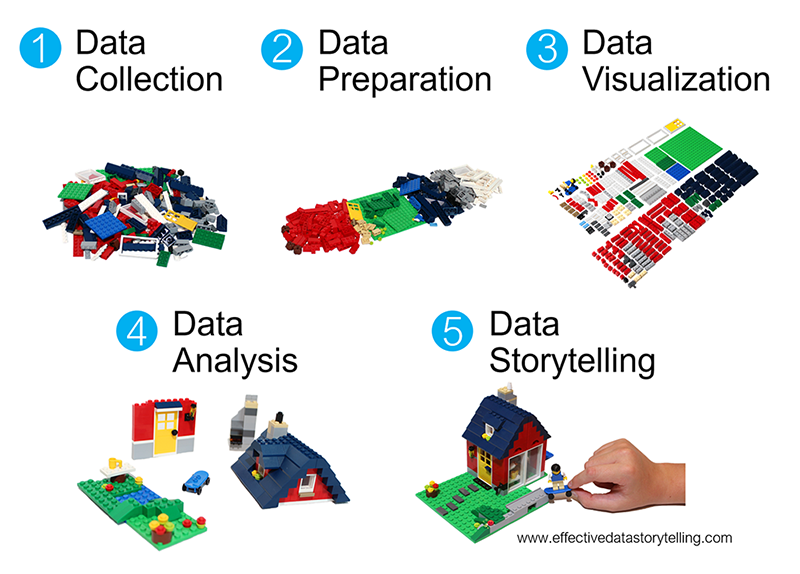
What's coming up?
- In the last \~4 weeks we'll focus on data storytelling through the completion of a course project.
- In the next \~1 week we'll address the other gaps in the workflow: data collection and analysis. We'll do so in the context of starting a data project...
\
\
\
\
**Starting a data project**
1. data collection\
Thus far in our data investigations, you've either been given data, or used TidyTuesday data. In this unit:
- We *will* explore how to find data, save data, import this data into RStudio, and do some preliminary data cleaning.
- We *won't* discuss how to collect data from scratch (e.g. via experiment, observational study, or survey).
2. data analysis\
Once we have data, we need to do some analysis. In this unit...
- We *will* bring together our wrangling & visualization tools to discuss **exploratory data analysis (EDA)**. EDA is the process of getting to know our data, obtaining insights from data, and using these insights to formulate, refine, and explore research questions.
- We will *not* explore other types of analysis, such as modeling & prediction. Take STAT 155 and 253 to learn more about these topics.
\
\
\
\
## Warm-up
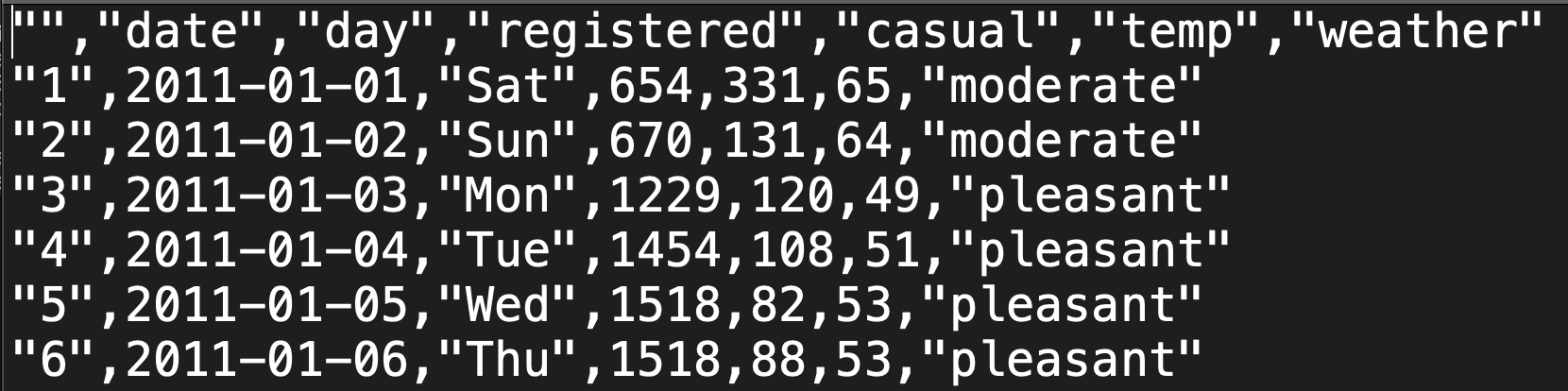
Before exploring how to find, store, import, check, and clean data, it's important to recognize that **data can be stored in various formats**. We've been working with `.csv` files. In the background, these have "comma-separated values" (csv):
\
{width="50%"}
\
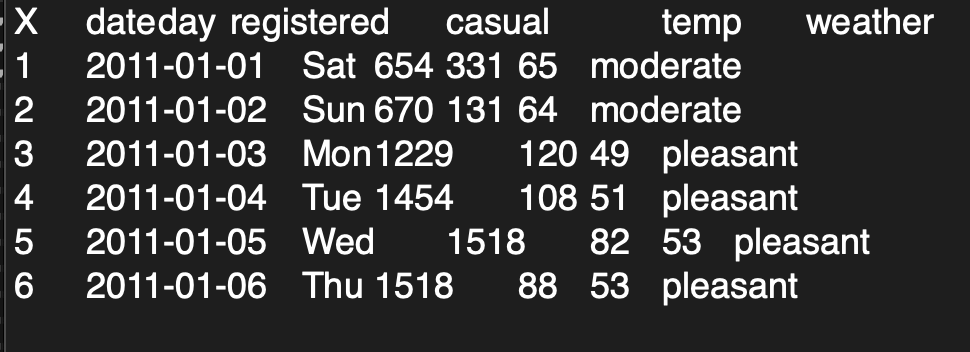
But there are many other common file types. For example, the following are compatible with R:
- Excel files: `.xls`, `.xlsx`
- R "data serialization" files: `.rds`
- files with tab-separated values: `.tsv`
{width="50%"}
\
\
\
\
### STEP 1: Finding data files {.unnumbered}
Data repositories are best when you're not looking for specific data. Here are just a few:
- TidyTuesday
- [awesome-public-datasets](https://github.com/caesar0301/awesome-public-datasets) (includes links to other data repositories at the end)
- [Kaggle](https://www.kaggle.com/datasets)
- [data.world](https://data.world/)
- [ProPublica](https://www.propublica.org/datastore/datasets)
- [sports data collection by Ohio State U](https://sportsandsociety.osu.edu/sports-data-sets)
But when we're searching for more specific data, search engines like Google are typically better. For example, try searching for:
`pet adoption data`
The word *data* is very broad! Matches could include articles that just have some simple statistics. For *data* in the sense that we mean it, e.g. a data *table*, we can use a more specific search:
`pet adoption filetype:csv`
You could also try other common file types that are compatible with R: `.tsv`, `.xls`, `.xlsx`, `.rds`
\
\
\
\
### STEP 2: Saving a local copy of the data file {.unnumbered}
Unless we're just doing a quick, one-off data analysis, it's important to store a local copy of a data file, i.e. save the data file to our own machine.
Mainly, we shouldn't rely on another person / institution to store a data file online, in the same place, forever!
Hot tips: Save your data...
- in a nice format (e.g. as a csv file)
- where you'll be able to find it again
- ideally, within a folder that's *dedicated* to the related project / assignment
- alongside the Rmd file(s) where you'll record your analysis of the data
\
\
\
\
### STEP 3: Importing the data file into RStudio {.unnumbered}
Once we have a local copy of our data file, we need to get it into RStudio! This process depends on 2 things: (1) the file *type* (e.g. .csv); and (2) the file *location*, i.e. where it's stored on your computer.
\
\
**1. FILE TYPE**
The file type indicates which *function* we'll need to import it. The table below lists some common import functions and when to use them.
| Function | Data file type |
|----------------|-------------------------------------------------------|
| `read_csv()` | .csv - you can save Excel files and Google Sheets as .csv |
| `read_delim()` | other delimited formats (tab, space, etc.) |
| `read_sheet()` | Google Sheet |
| `st_read()` | spatial data shapefile |
NOTE: In comparison to `read.csv`, `read_csv` is faster when importing large data files and can more easily parse complicated datasets (e.g. with dates, times, percentages).
\
\
**2. FILE LOCATION**
To import the data, we apply the appropriate function from above to the **file path**.
A file path is an address to where the file is stored on our computer.
Consider "1600 Grand Ave, St. Paul, MN 55105". Think about how different parts of the address give increasingly more specific information about the location. "St. Paul, MN 55105" tells us the city and smaller region within the city, "Grand Ave" tells us the street, and "1600" tells us the specific location on the street.
In the example below, the file path tells us the location giving more and more specific information as you read it from left to right.
- "\~" on an Apple computer tells you that you are looking in the user's home directory.
- "Desktop" tells you to go to the Desktop within that home directory.
- "112" tells you that you are looking in the 112 folder on the Desktop.
- "data" tells you to next go in the data folder in the 112 folder.
- "my_data.csv" tells you that you are looking for a file called my_data.csv located within the data folder.
```{r eval = FALSE}
library(tidyverse)
my_data <- read_csv("~/Desktop/112/data/my_data.csv")
```
\
\
\
\
### STEP 4: Preliminary data checks and cleaning {.unnumbered}
Once the data is loaded, ask yourself a few questions:
What's the structure of the data?
- Use `str()` to learn about the numbers of variables and observations as well as the classes or types of variables (date, location, string, factor, number, boolean, etc.)
- Use `head()` to view the top of the data table
- Use `View()` to view the data in a spreadsheet-like viewer
Is there anything goofy that we need to clean before we can analyze the data?
- Is it in a tidy format?
- How many rows are there? What does the row mean? What is an observation?
- Is there consistent formatting for categorical variables?
- Is there missing data that needs to be addressed?
\
\
\
\
### STEP 5: Understanding the data {.unnumbered}
Start by understanding the data that is available to you. If you have a codebook, you have struck gold! If not (the more common case), you'll need to do some detective work that often involves talking to people.
At this stage, ask yourself:
- Where does my data come from? How was it collected?[^15-data-import-notes-1]
- Is there a codebook? If not, how can I learn more about it?
- Are there people I can reach out to who have experience with this data?
[^15-data-import-notes-1]: Particularly important questions about how it was collected include WHO (whether it is a sample of a larger data set, and, if so, how the sampling was done? Randomly? All cases during a specific time frame? All data for a selected set of users?), WHEN (is this current data or historical? what events may have had an impact?), WHAT (what variables were measured? how was it measured, self-reported through a questionnaire or measured directly?), WHY (who funded the data collection? for what purposes what the data collected? to whose benefit was the data collected?) Answers to such questions strongly impact the conclusions you will be able to draw from the data.
## Exercises
Suppose our goal is to work with data on movie reviews, and that we've already gone through the work to find a dataset. The "imdb_5000_messy.csv" file is posted on Moodle. Let's work with it!
\
\
\
\
### Exercise 1: Save a local copy of the data file {.unnumbered}
#### Part a {.unnumbered}
On your laptop (or in the RStudio server):
- Download the "imdb_5000_messy.csv" file.
- Move it to / save it in the *data* folder that you created at the beginning of class. (e.g. Desktop \> 112 folder \> IMDB folder \> data folder)
#### Part b {.unnumbered}
Tip: After saving your data file, it's important to record appropriate citations and info in either a new qmd (eg: "imdb_5000_messy_README.qmd") or in the qmd where you'll analyze the data. These citations should include:
- the data *source*, i.e. where you *found* the data
- the data *creator*, i.e. who / what group *collected* the original data
- possibly a data *codebook*, i.e. descriptions of the data variables
To this end, check out where we originally got our IMDB data:
https://www.kaggle.com/datasets/tmdb/tmdb-movie-metadata
After visiting that website, take some quick notes here on the data *source* and *creator*.
\
\
\
\
### Exercise 2: Import the data into RStudio {.unnumbered}
Let's get the local copy of our data file into RStudio! Remember that this process depends on 2 things: the file *type* and *location*. Since our file *type* is a csv, we can import it using `read_csv()`. But we have to supply the file *location* through a file path. We can either use an **absolute file path** or a **relative file path**.
#### Part a {.unnumbered}
An absolute file path describes the location of a file starting from the root or home directory. How we refer to this directory depends upon your machine:
- On a Mac: `~`
- On Windows: typically `C:\`
- On the RStudio server: `~`
Then the complete file path to the IMDB data file, in the IMDB folder, in the 112 folder, on your desktop also depends upon your machine:
- On a Mac: `~/Desktop/112/IMDB/data/imdb_5000_messy.csv`
- On Windows: `C:\Desktop\112\IMDB\data\imdb_5000_messy.csv` or `C:\\Desktop\\112\\IMDB\\data\\imdb_5000_messy.csv`
- On the server: `~/112/IMDB/data/imdb_5000_messy.csv`
Putting this together, use `read_csv()` with the appropriate absolute file path to import your data into RStudio. Save this as `imdb_messy`.
```{r}
library(tidyverse)
# imdb_messy <- read_csv("___")
```
#### Part b {.unnumbered}
Absolute file paths can get really long! Further, since *your* absolute files path are specific to *your* machine, they make it complicated to share code with collaborators. A **relative file path** describes the location of a file from the current "working directory", i.e. where RStudio would currently look for / save files on your computer. Check what your working directory is *inside this Rmd*:
```{r}
# This should be the folder where you stored this Rmd!
getwd()
```
Next, check what the working directory is for the *console* by typing `getwd()` in the *console*. This is probably different, meaning that the relative file paths that will work in your Rmd won't work in the console! You can either exclusively work inside your Rmd, or change the working directory in your console, by navigating to the following in the upper toolbar: Session \> Set Working Directory \> To Source File location.
#### Part c {.unnumbered}
As is good practice, we created a folder for our analysis (`IMDB`) that includes *both*:
- the .qmd with our analysis (`imdb_analysis.qmd`)
- a `data` folder with our data file (`imdb_5000_messy.csv`)
Since these files live in the same working directory, we don't have to write out *absolute file paths* that go all the way to the root directory. We can use *relative file paths* that only go back to the working directory, here our IMDB folder:
- On a Mac: `./data/imdb_5000_messy.csv`
- On Windows: `.\data\imdb_5000_messy.csv` or `.\\data\\imdb_5000_messy.csv`
- On the server: `./data/imdb_5000_messy.csv`
NOTE: You might need `..` if the working directory ends with `IMDB/` instead of `IMDB`.
Putting this together, use `read_csv()` with the appropriate relative file path to import your data into RStudio. Save this as `imdb_temp` (`temp` for "temporary"). Convince yourself that this worked, i.e. you get the same dataset as `imdb_messy`.
```{r}
#imdb_temp <- read_csv("___")
```
#### Part d: OPTIONAL {.unnumbered}
Sometimes, we don't want to import the *entire* dataset. For example, we might want to...
- skips some rows (eg: if they're just "filler")
- only import the *first* "n" rows (eg: if the dataset is really large)
- only import a *random* subset of "n" rows (eg: if the dataset is really large)...
The "data import cheat sheet" at the top of this Rmd, or Google, are handy resources here. As one example...
```{r}
# Try importing only the first 5 rows
# read_csv("___", n_max = ___)
```
\
\
\
\
### Exercise 3: Preliminary data checks {.unnumbered}
After importing new data into RStudio, you MUST do some quick checks of the data. Here are two first steps that are especially useful.
#### Part a {.unnumbered}
Open `imdb_messy` in the spreadsheet-like viewer by typing `View(imdb_messy)` in the console. Sort this "spreadsheet" by different variables by clicking on the arrows next to the variable names. Do you notice anything unexpected?
#### Part b {.unnumbered}
Do a quick `summary()` of each variable in the dataset. *One* way to do this is below:
```{r}
# imdb_messy %>%
# mutate(across(where(is.character), as.factor)) %>% # convert characters to factors in order to summarize
# summary()
```
Follow-up:
- What type of info is provided on quantitative variables?
- What type of info is provided on categorical variables?
- What stands out to you in these summaries? Is there anything you'd need to clean before using this data?
\
\
\
\
### Exercise 4: Preliminary cleaning -- factor variables 1 {.unnumbered}
If you didn't already in Exercise 3, check out the `color` variable in the `imdb_messy` dataset.
- More specifically, what different categories does the `color` variable take, and how many movies fall into each of these categories?
```{r}
```
- What's goofy about this / what do we need to fix?
\
\
\
\
### Exercise 5: Preliminary cleaning -- factor variables 2 {.unnumbered}
When working with categorical variables like `color`, the categories must be "clean", i.e. consistent and in the correct format. Let's make that happen.
#### Part a {.unnumbered}
We *could* open the .csv file in, say, Excel or Google sheets, clean up the `color` variable, save a clean copy, and then reimport that into RStudio. BUT that would be the wrong thing to do. Why is it important to use R code, which we then save inside this Rmd, to clean our data?
#### Part b {.unnumbered}
Let's use R code to change the `color` variable so that it appropriately combines the various categories into only 2: `Color` and `Black_White`. We've learned a couple sets of string-related tools that could be handy here. First, starting with the `imdb_messy` data, change the `color` variable using one of the functions we learned in Activity 12:
`fct_relevel()`, `fct_recode()`, `fct_reorder()`
Store your results in `imdb_temp` (don't overwrite `imdb_messy`). To check your work, print out a `count()` table of the `color` variable in `imdb_temp`.
```{r}
```
#### Part c {.unnumbered}
Repeat Part b using one of our string functions from Activity 14:
`str_replace()`, `str_replace_all()`, `str_to_lower()`, `str_sub()`, `str_length()`, `str_detect()`
```{r}
```
\
\
\
\
### Exercise 6: Preliminary cleaning -- missing data 1 {.unnumbered}
Throughout these exercises, you've probably noticed that there's a bunch of missing data. This is encoded as `NA` (not available) in R. There are a few questions to address about missing data:
- *How many* values are missing data? What's the volume of the missingness?
- *Why* are some values missing?
- *What* should we do about the missing values?
Let's consider the first 2 questions in this exercise.
#### Part a {.unnumbered}
As a first step, let's simply understand the *volume* of NAs. Specifically:
```{r}
# Count the total number of rows in imdb_messy
#___(imdb_messy)
# Then count the number of NAs in each column
#colSums(is.na(imdb_messy))
```
#### Part b {.unnumbered}
As a second step, let's think about *why* some values are missing. Study the individual observations with NAs carefully. Why do you think they are missing? Are certain films more likely to have more NAs than others?
#### Part c {.unnumbered}
Consider a more specific example. Obtain a dataset of movies that are missing data on `actor_1_facebook_likes`. Then explain why you think there are NAs. HINT: `is.na(___)`
```{r}
```
\
\
\
\
### Exercise 7: Preliminary cleaning -- missing data 2 {.unnumbered}
Next, let's think about what to *do* about the missing values. There is no perfect or universal approach here. Rather, we must think carefully about...
- why the values are missing
- what we want to do with our data
- the impact of removing or replacing missing data on our work / conclusions
#### Part a {.unnumbered}
Calculate the average duration of a film. THINK: How can we deal with the NA's?
```{r}
```
Follow-up:
How are the NAs dealt with here? Did we have to create and save a new dataset in order to do this analysis?
#### Part b {.unnumbered}
Try out the `drop_na()` function:
```{r}
# imdb_temp <- drop_na(imdb_messy)
```
Follow-up questions:
- What did `drop_na()` do? How many data points are left?
- In what situations might this function be a good idea?
- In what situations might this function be a bad idea?
#### Part c {.unnumbered}
`drop_na()` removes data points that have *any* NA values, even if we don't care about the variable(s) for which data is missing. This can result in losing a lot of data points that *do* have data on the variables we actually care about! For example, suppose we only want to explore the relationship between film `duration` and whether it's in `color`. Check out a plot:
```{r}
# ggplot(imdb_messy, aes(x = duration, fill = color)) +
# geom_density()
```
Follow-up:
- Create a new dataset with *only* and *all* movies that have complete info on `duration` and `color`. HINT: You could use `!is.na(___)` or `drop_na()` (differently than above)
- Use this new dataset to create a new and improved plot.
- How many movies remain in your new dataset? Hence why this is better than using the dataset from part b?
```{r}
```
#### Part d {.unnumbered}
In some cases, missing data is more *non*-data than *unknown* data. For example, the films with NAs for `actor_1_facebook_likes` actually have *0* Facebook likes -- they don't even have actors! In these cases, we can *replace* the NAs with a 0. Use the `replace_na()` function to create a new dataset (`imdb_temp`) that replaces the NAs in `actor_1_facebook_likes` with 0. You'll have to check out the help file for this function.
```{r}
```
\
\
\
\
### Exercise 8: New data + projects {.unnumbered}
Let's practice the above ideas while also planting some seeds for the course project, which will be done in groups. Each group will pick and analyze their own dataset. The people you're sitting with today aren't necessarily your project groups! BUT do some brainstorming together:
- Share with each other: What are some personal hobbies or passions or things you've been thinking about or things you'd like to learn more about? Don't think too hard about this! Just share what's at the top of mind today.
- Each individual: Find a dataset online that's related to one of the topics you shared in the above prompt.
- Discuss what data you found with your group!
- Load the data into RStudio, perform some basic checks, and perform some preliminary cleaning, as necessary.
\
\
\
\