---
title: "Variable Selection - Part 1 (Notes)"
subtitle: "Stat 253"
author: "Your Name"
format:
html:
toc: true
toc-depth: 2
embed-resources: true
---
```{r setup}
#| include: false
knitr::opts_chunk$set(
collapse = TRUE,
warning = FALSE,
message = FALSE,
error = TRUE,
fig.height = 2.75,
fig.width = 4.25,
fig.env='figure',
fig.pos = 'h',
fig.align = 'center')
```
# Notes: Model Selection {-}
## Context {.unnumbered .smaller}
{width=100%}
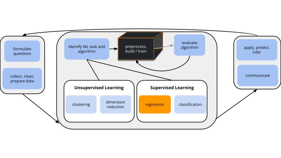
- **world = supervised learning**
We want to model some output variable $y$ using a set of *potential* predictors ($x_1, x_2, ..., x_p$).
- **task = regression**
$y$ is quantitative
- **model = linear regression**
We'll assume that the relationship between $y$ and ($x_1, x_2, ..., x_p$) can be represented by
$$y = \beta_0 + \beta_1 x_1 + \beta_2 x_2 + ... + \beta_p x_p + \varepsilon$$
\
## Inferential v. Predictive Models {.unnumbered .smaller}
In model building, the decision of which predictors to use **depends upon our goal**.
**Inferential models**
- Goal: Explore & test hypotheses about a specific relationship.
- Predictors: Defined by the goal.
- Example: An economist wants to understand how salaries ($y$) vary by age ($x_1$) while controlling for education level ($x_2$).
:::{.callout-note title="STAT 155 Review"}
What techniques did you discuss in STAT 155 for selecting which variables to
put in your model?
:::
\
**Predictive models**
::: incremental
- Goal: Produce the "best" possible predictions of $y$.
- Predictors: Any combination of predictors that help us meet this goal.
- Example: A mapping app wants to provide users with quality estimates of arrival time ($y$) utilizing any useful predictors (eg: time of day, distance, route, speed limit, weather, day of week, traffic radar...)
:::
\
## Model Selection Goals {.unnumbered .smaller}
**Model selection** algorithms can *help* us build a **predictive model** of $y$ using a set of potential predictors ($x_1, x_2, ..., x_p$).
There are 3 general approaches to this task:
:::incremental
1. **Variable selection (today)**
Identify a *subset* of predictors to use in our model of $y$.
2. **Shrinkage / regularization (next class)**
*Shrink* / regularize the coefficients of all predictors toward or to 0.
3. **Dimension reduction (later in the semester)**
*Combine* the predictors into a smaller set of new predictors.
:::
# Exercises: Part 1 {-}
## Instructions {.unnumbered .smaller}
*As a group*, you'll design a **variable selection algorithm** to pick which
predictors to use in a predictive model of `height`.
Specifically, you will:
- come up with one algorithm, document it, and try it (15 mins)
- try another group's algorithm (5 mins)
NOTE: This will NOT be perfect! Our goals are to:
- Have fun and work together!
- Tap into your *intuition* for key questions and challenges in variable selection.
- *Deepen* your understanding of "algorithms" and "tuning parameters" by designing and communicating your own.
\
## Questions {.unnumbered .smaller}
Let's build a **predictive model** of `height` in inches using one or more of 12 possible predictors. Other than `age` and `weight`, these are circumferences measured in cm.
```{r}
#| message: false
#| warning: false
#| eval: true
# Load packages
library(tidyverse)
library(tidymodels)
# Load data
humans <- read.csv("https://mac-stat.github.io/data/bodyfat1.csv")
names(humans)
```
\
A **heat map** displays correlations for each pair of variables in our dataset. Not only is `height` correlated with multiple predictors, the predictors are correlated with one another (mulicollinear)! We don't need *all* of them in our model.
```{r fig.width = 6, fig.height = 6}
#| eval: true
#| code-fold: true
# Get the correlation matrix
library(reshape2)
cor_matrix <- cor(humans)
cor_matrix[lower.tri(cor_matrix)] <- NA
cor_matrix <- cor_matrix %>%
melt() %>%
na.omit() %>%
rename(correlation = value)
# Visualize the correlation for each pair of variables
ggplot(cor_matrix, aes(x = Var1, y = Var2, fill = correlation)) +
geom_tile(color = "white") +
scale_fill_gradient2(
low = "blue", high = "red", mid = "white",
midpoint = 0, limit = c(-1,1)) +
labs(x = "", y = "") +
theme_minimal() +
theme(axis.text.x = element_text(angle = 60, hjust = 1)) +
coord_fixed()
```
1. **Design your own algorithm (15 minutes)**
- Do not use any materials from outside this class.
- Document your algorithm in words (not code) in this [google doc](https://docs.google.com/document/d/1OD1Xv6SFp9pgxSDEB_PKuOzy83xEaFvJZHhLaYf2Nqc/edit?usp=sharing).
- Your algorithm must:
- be *clear* to other humans
- be clear to a *machine* (cannot utilize context)
- lead to a *single* model that uses 0-12 of our predictors
- define and provide directions for selecting any tuning parameters
- Implement as many steps of your algorithm as possible in the time allotted. You can modify the code below to build and evaluate the models in your algorithm:
```{r eval = FALSE}
# STEP 1: model specification
lm_spec <- linear_reg() %>%
set_mode("regression") %>%
set_engine("lm")
# STEP 2: model estimation
height_model_1 <- lm_spec %>%
fit(height ~ age + weight + neck + chest + abdomen + hip + thigh + knee + ankle + biceps + forearm + wrist, data = humans)
# Check it out
height_model_1 %>%
tidy()
# CV MAE
set.seed(253)
lm_spec %>%
fit_resamples(
height ~ age + weight + neck + chest + abdomen + hip + thigh + knee + ankle + biceps + forearm + wrist,
resamples = vfold_cv(humans, v = 10),
metrics = metric_set(mae)
) %>%
collect_metrics()
```
2. **Test another group's algorithm (5 minutes)**
Try to implement the next algorithm below yours (or the first algorithm if your group's is last). Think: Are the steps clear? What are the drawbacks to the algorithm? *Leave any comments you have for the group in the google doc.*
# Done!
- Render your notes.
- Check the solutions in the course website (Solution drop downs).
- If you finish all that during class, start your homework!