Topic 8 Interaction Models

Learning Goals

Understand what research questions can be answered with interaction models
Interpret coefficients in interaction models
Connect visualizations to the coefficient estimates in interaction models
Graphically/geometrically describe the “pictures” implied by different types of interaction models

Discussion and Exercises

A template RMarkdown document that you can start from is available here.

We will continue looking at the diamonds dataset.

carat: the weight of the diamond in carats (1 carat = 200 milligrams)
price: price in US dollars
cut: quality of the cut of the diamond (Fair, Good, Very Good, Premium, Ideal)
color: Level 1 (best) to Level 7 (worst)
clarity: Level 1 (worst) to Level 8 (best)
x, y, and z: length, width, and depth respectively (in mm)
depth: total depth percentage = z / mean(x, y)
table: width of top of diamond relative to widest point

library(readr)
library(ggplot2)
library(dplyr)

diamonds <- read_csv("https://www.dropbox.com/s/9c8jqda4pwaq8i1/diamonds.csv?dl=1")

Warm-up: Consider the model of price as a function of clarity and carat.

\[ E[\hbox{price}] = \beta_0 + \beta_1\hbox{clarityLevel_2} + \beta_2\hbox{clarityLevel_3} + \cdots + \beta_7\hbox{clarityLevel_8} + \beta_8\hbox{carat} \]

Why was this called a parallel lines model?
Draw a picture of the relationships that this model implies and label the picture with the coefficients of the model.

Exercise 1: We looked at a scatterplot of price versus carat and boxplots of price versus clarity, but we haven’t looked at all three variables simultaneously. Let’s enrich the scatterplot to additionally show clarity.

We’ve seen that we can have x, y, color, and fill aesthetics (inside the aes()). How might we adapt the code below to show different color trend lines corresponding to the 8 clarity levels?

ggplot(diamonds, aes(x = carat, y = price)) +
    geom_point() +
    geom_smooth()

If the relationship between the response $y$ and predictor $x_1$ differs depending on the value / categories of another predictor $x_2$, we say that $x_1$ and $x_2$ interact. We capture this in our models with an interaction term: $x_1 \times x_2$.

\[ E[y] = \beta_0 + \beta_1 x_1 + \beta_2 x_2 + \beta_3 x_1 \times x_2 \]

The coefficient $\beta_3$ in front of the interaction term is called the interaction coefficient.

For now, let’s work with a subset of the data that just has two clarity levels.

\[ E[\hbox{price}] = \beta_0 + \beta_1\hbox{clarity2} + \beta_2\hbox{carat} + \beta_3\hbox{clarity2}\times\hbox{carat} \]

diamonds_sub <- diamonds %>%
    filter(clarity %in% c("Level_1", "Level_2"))

mod1 <- lm(price ~ clarity*carat, data = diamonds_sub)
summary(mod1)

## 
## Call:
## lm(formula = price ~ clarity * carat, data = diamonds_sub)
## 
## Residuals:
##     Min      1Q  Median      3Q     Max 
## -6051.1  -645.7  -112.8   485.6  6304.1 
## 
## Coefficients:
##                      Estimate Std. Error t value Pr(>|t|)    
## (Intercept)          -1480.56     103.76  -14.27   <2e-16 ***
## clarityLevel_2       -1937.78     108.04  -17.94   <2e-16 ***
## carat                 4209.79      72.51   58.06   <2e-16 ***
## clarityLevel_2:carat  3660.46      76.76   47.69   <2e-16 ***
## ---
## Signif. codes:  0 '***' 0.001 '**' 0.01 '*' 0.05 '.' 0.1 ' ' 1
## 
## Residual standard error: 1247 on 9931 degrees of freedom
## Multiple R-squared:  0.911,  Adjusted R-squared:  0.9109 
## F-statistic: 3.387e+04 on 3 and 9931 DF,  p-value: < 2.2e-16

Note: When you see a colon between two variables, the colon means a multiplication sign. (clarityLevel_2:carat is the product of the clarityLevel_2 indicator variable and the carat variable.)

Model formula

\[ \begin{align*} E[\hbox{price}] &= \beta_0 + \beta_1\hbox{clarity2} + \beta_2\hbox{carat} + \beta_3\hbox{clarity2}\times\hbox{carat} \\ &= -1480.56 - 1937.78\,\hbox{clarity2} + 4209.79\,\hbox{carat} + 3660.46\,\hbox{clarity2}\times\hbox{carat} \end{align*} \]

Model formula for clarity level 1

\[ \begin{align*} E[\hbox{price}] &= -1480.56 - 1937.78\times 0 + 4209.79\,\hbox{carat} + 3660.46\times 0 \times\hbox{carat} \\ &= -1480.56 + 4209.79\,\hbox{carat} \end{align*} \]

Model formula for clarity level 2

\[ \begin{align*} E[\hbox{price}] &= -1480.56 - 1937.78\times 1 + 4209.79\,\hbox{carat} + 3660.46\times 1 \times\hbox{carat} \\ &= (-1480.56 - 1937.78) + (4209.79 + 3660.46)\,\hbox{carat} \\ &= -3418.34 + 7870.25\,\hbox{carat} \end{align*} \]

It is very helpful to draw a picture labeled with the coefficients.

Coefficient interpretations:

Intercept $\beta_0$: -1480.56
The average price for a zero carat, level 1 clarity diamond. (Could have made more meaningful by centering carat, but generally not interested in the intercept.)
$\beta_2$ for carat: 4209.79
The slope for the clarity level 1 model. On average, diamond price increases by $4209.79 per carat increase in level 1 clarity diamonds. (This rate of change is different for clarity level 2 diamonds.)
$\beta_1$ for clarityLevel_2: -1937.78
The change in y-intercept going from clarity level 1 to 2.
On average, zero carat diamonds that are clarity level 2 are worth $1937.78 less than zero carat, clarity level 1 diamonds.
$\beta_3$ for the interaction term (clarityLevel_2:carat): 3660.46
The change in slope for the clarity level 2 vs. the clarity level 1 model. The average change in price per carat increase is 3660.46 ($/carat) higher for clarity level 2 vs. clarity level 1 diamonds.
The slope is steeper for level 2. A carat is worth more for a level 2 clarity diamond.

Exercise 2: Fit a model with interaction between clarity and carat for the full diamonds dataset.

Write out the model formulas for clarity level 1, 2, … diamonds until you get the hang of it.
Draw a picture with the model lines for clarity level 1, 2, … 8 diamonds. Annotate this picture with the model coefficients.
Interpret the clarityLevel_3 and clarityLevel_3:carat coefficients. Repeat for level 4 and onwards until you get the hang of it.
For which clarity level is a carat worth the most? How much is a carat worth on average?

Exercise 3: Now let’s consider diamond color (Level 1 is best and Level 7 is worst).

What research question are you exploring when you fit a model with interaction between color and carat? Generalize this to a broader context.
Make a plot that allows you to explore potential interaction between color and carat. What are you looking to see in the plot? Do you think an interaction model is appropriate?
Fit the interaction model, and focus on the coefficients of substantive interest. Summarize your overall conclusions.

The remainder of these exercises don’t require R.

Exercise 4: We’ve seen interaction between a categorical and a quantitative variable. Two categorical variables can interact as well. Consider the model

\[ \begin{align*} E[\hbox{winpercent}] = \beta_0 &+ \beta_1\hbox{chocolateTRUE} \\ &+ \beta_2\hbox{peanutyalmondyTRUE} + \beta_3\hbox{chocolateTRUE}\times\hbox{peanutyalmondyTRUE} \end{align*} \]

Write out the model formulas for the non-chocolate candies and for the chocolate candies. Leave peanutyalmondyTRUE as-is without plugging in anything for it. (Similar to leaving carat as-is in the diamonds context.)
From part (a), interpret $\beta_0$ and $\beta_2$. Then interpret $\beta_0+\beta_1$ and $\beta_2+\beta_3$.

The mean winpercents in all four combinations of chocolate and peanutyalmondy are shown below. From this information, determine the values of the model coefficients.

candy %>%
    dplyr::group_by(chocolate, peanutyalmondy) %>%
    summarize(mean_winpercent = mean(winpercent))

## `summarise()` has grouped output by 'chocolate'. You can override using the `.groups` argument.

## # A tibble: 4 x 3
## # Groups:   chocolate [2]
##   chocolate peanutyalmondy mean_winpercent
##   <lgl>     <lgl>                    <dbl>
## 1 FALSE     FALSE                     42.5
## 2 FALSE     TRUE                      34.9
## 3 TRUE      FALSE                     57.3
## 4 TRUE      TRUE                      68.5

Now interpret $\beta_0$, $\beta_2$, $\beta_0+\beta_1$, and $\beta_2+\beta_3$ in a contextually meaningful way. Is nuttiness (peanutyalmondy) “better” in chocolate candies or in non-chocolate candies?

Exercise 5: Two quantitative variables can interact as well. In a model of Price, the Mileage and Age of a used car interact: the relationship between mileage and price differs depending upon the age of the car. Below, the yellow lines represent the relationship between price and mileage for 1 year old, 5 year old, and 10 year old used cars.

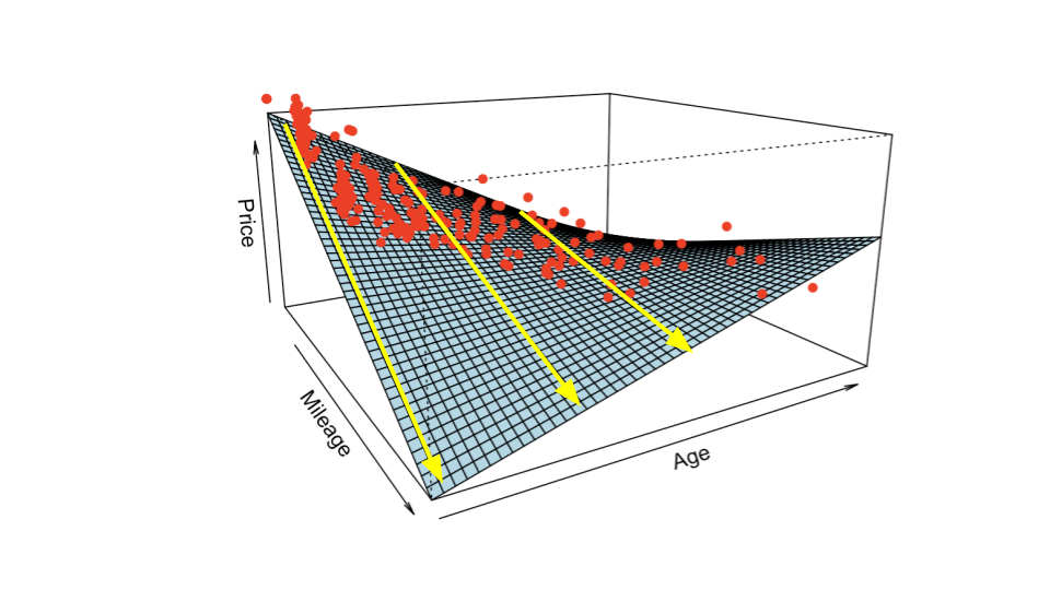
Based on this plot, what do you anticipate about the signs of the coefficients in the interaction model? (Don’t look ahead to the output below yet.)

\[ E[\hbox{Price}] = \beta_0 + \beta_1 \hbox{Age} + \beta_2 \hbox{Mileage} + \beta_3 \hbox{Age}\times\hbox{Mileage} \]

Based on the model output below, write the model formulas relating Price to Mileage for cars that are 0 years (new), 5 years, and 12 years old.

fords <- read_csv("https://www.dropbox.com/s/wmb6ktyaw5c5jwf/Fords.csv?dl=1")
fords_mod <- lm(Price ~ Age*Mileage, data = fords)
summary(fords_mod)

## 
## Call:
## lm(formula = Price ~ Age * Mileage, data = fords)
## 
## Residuals:
##     Min      1Q  Median      3Q     Max 
## -6950.1 -1254.4   -35.5  1124.6  7355.2 
## 
## Coefficients:
##               Estimate Std. Error t value Pr(>|t|)    
## (Intercept)  1.932e+04  2.256e+02   85.65   <2e-16 ***
## Age         -1.523e+03  6.042e+01  -25.21   <2e-16 ***
## Mileage     -1.349e-01  4.835e-03  -27.91   <2e-16 ***
## Age:Mileage  1.320e-02  6.488e-04   20.34   <2e-16 ***
## ---
## Signif. codes:  0 '***' 0.001 '**' 0.01 '*' 0.05 '.' 0.1 ' ' 1
## 
## Residual standard error: 1899 on 606 degrees of freedom
##   (25 observations deleted due to missingness)
## Multiple R-squared:  0.8342, Adjusted R-squared:  0.8334 
## F-statistic:  1016 on 3 and 606 DF,  p-value: < 2.2e-16

Given (b), what does the interaction coefficient help us learn about the relationship between Price and Mileage?
Extra (not required but good practice): Interpret each of the coefficients in the above model.

Interlude: Take a moment to think about the theme of these interaction exercises. In all of them, we have used interaction terms to describe how the relationship between a variable and the response is modified by the value of another variable. For this reason, interaction is also called effect modification.

Diamond clarity and color modify the effect of size on price. Note that effect modification/interaction is symmetric, so we can also say that diamond size modifies the effect of clarity and color on price. However, usually with interaction between a quantitative and a categorical variable, we describe it in the first way.
Chocolatiness modifies the effect of nuttiness on candy popularity. Symmetrically, nuttiness modifies the effect of chocolatiness on candy popularity.
Car age modifies the effect of mileage on price. Symmetrically, mileage modifies the effect of care age on its price.

Exercise 6: Confounding and interaction are not the same idea.

Draw or describe how the situation below could arise:
- carat does confound the relationship between clarity and price.
- There is no interaction between carat and clarity.
Draw or describe how the situation below could arise:
- carat does not confound the relationship between clarity and price.
- There is interaction between carat and clarity.