Topic 6 Modeling Concepts (Part 2)

Learning Goals

Practice simple linear regression modeling concepts: model formula, coefficient interpretations, predicted values, residuals
Develop two ideas of model quality: $R^2$ and residual standard error
Understand how categorical predictors are incorporated in linear regression models

Warm-up

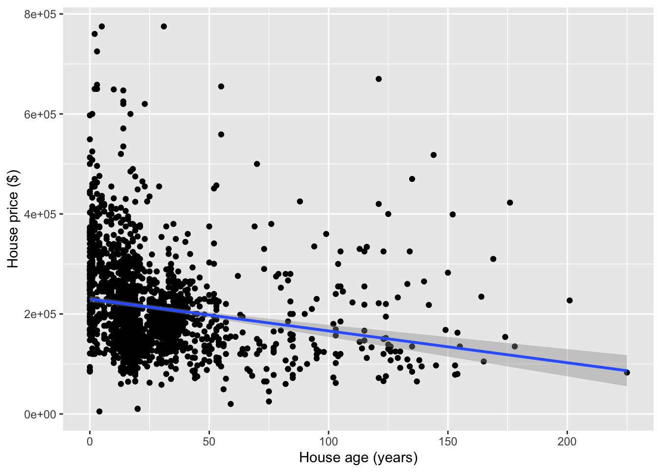
mod1 <- lm(Price ~ Age, data = homes)
summary(mod1)

## 
## Call:
## lm(formula = Price ~ Age, data = homes)
## 
## Residuals:
##     Min      1Q  Median      3Q     Max 
## -222183  -66299  -22232   43147  564995 
## 
## Coefficients:
##              Estimate Std. Error t value Pr(>|t|)    
## (Intercept) 229728.46    3218.18  71.385  < 2e-16 ***
## Age           -636.26      79.66  -7.987  2.5e-15 ***
## ---
## Signif. codes:  0 '***' 0.001 '**' 0.01 '*' 0.05 '.' 0.1 ' ' 1
## 
## Residual standard error: 96700 on 1726 degrees of freedom
## Multiple R-squared:  0.03564,    Adjusted R-squared:  0.03508 
## F-statistic: 63.79 on 1 and 1726 DF,  p-value: 2.502e-15

Write the regression model formula using numbers from this output.
Interpret all coefficients in this model.
For a 50 year old house whose price is $100,000, what is the residual?

Discussion

What can we quantify about residuals to measure model quality?

Not the sum or the mean of residuals (will always be zero)
Residual standard error: essentially equal to the standard deviation of the residuals
Scale of residual standard error changes with the scale of the data (e.g., house prices versus strength-to-weight ratio)
- Can we put the variance of the residuals on a nicer scale? Say from 0 to 1? Yes, we can.
Some facts:

\[ \hbox{Var}(\hbox{response}) = \hbox{Var}(\hbox{residuals}) + \hbox{Var}(\hbox{predicted values}) \] \[ \hbox{Total variation} = \hbox{Unexplained variation} + \hbox{Explained variation} \]

$R^2$: What fraction of total variation in the response is explained by the model?
- Hopefully a lot. Which would mean that there is relatively little unexplained variation.
- Ranges from 0 to 1

\[ \begin{align*} R^2 &= \frac{\hbox{Var}(\hbox{predicted values})}{\hbox{Var}(\hbox{response})} \\ &= 1 - \frac{\hbox{Var}(\hbox{residuals})}{\hbox{Var}(\hbox{response})} \end{align*} \]

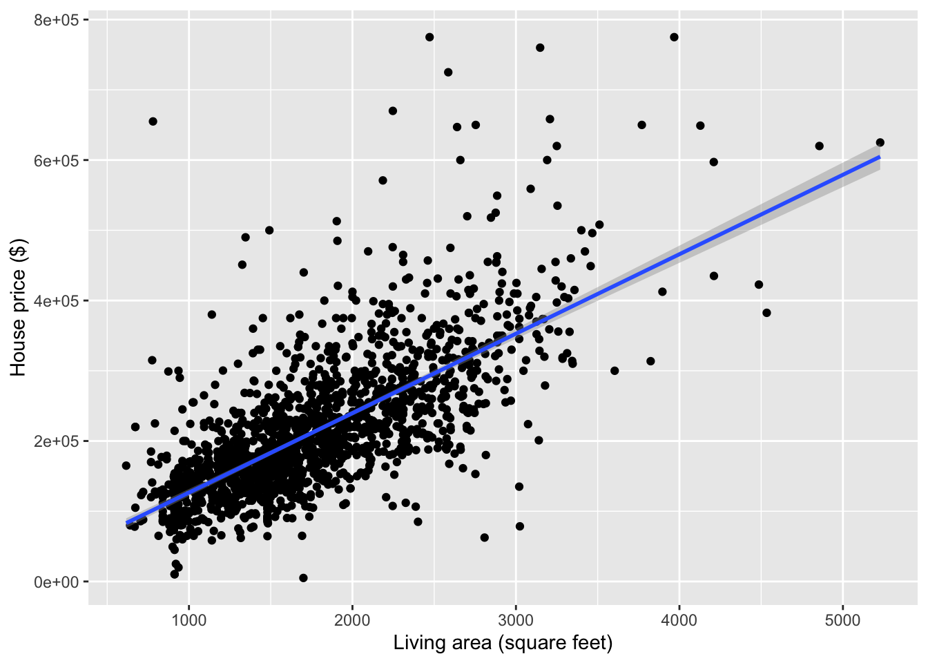
mod1 <- lm(Price ~ Living.Area, data = homes)
summary(mod1)

## 
## Call:
## lm(formula = Price ~ Living.Area, data = homes)
## 
## Residuals:
##     Min      1Q  Median      3Q     Max 
## -277022  -39371   -7726   28350  553325 
## 
## Coefficients:
##              Estimate Std. Error t value Pr(>|t|)    
## (Intercept) 13439.394   4992.353   2.692  0.00717 ** 
## Living.Area   113.123      2.682  42.173  < 2e-16 ***
## ---
## Signif. codes:  0 '***' 0.001 '**' 0.01 '*' 0.05 '.' 0.1 ' ' 1
## 
## Residual standard error: 69100 on 1726 degrees of freedom
## Multiple R-squared:  0.5075, Adjusted R-squared:  0.5072 
## F-statistic:  1779 on 1 and 1726 DF,  p-value: < 2.2e-16

Residual standard error: $69100
- This describes the amount of spread in the residuals.
- What qualifies as “high”? Imagine that your residual changed by that much. Is that a lot?
$R^2$ (Multiple R-squared): 0.5075
- 50.75% of the variation in house prices is explained by a simple linear regression model with square footage as a predictor
- What qualifies as “high”? Context helps determine if the response variable simply varies a lot. (e.g., stocks)

How do we incorporate categorical predictors?

In our housing dataset, there is a Heat.Type that indicates whether the heating type of the house is of type 2, 3, or 4.

Including a categorical predictor variable creates $L-1$ indicator variables where $L$ is the number of levels of the categorical variable.

Type 2 is chosen as the reference category by default in R because it is first in alphanumeric order.
Heat.Type3 and Heat.Type4 get created as indicator variables by taking the original variable name (Heat.Type) and pasting the name of the category (3 or 4 afterward)
- Heat.Type3 equals 1 is this case is of heating type 3. Equals 0 otherwise.
- Heat.Type4 equals 1 is this case is of heating type 4. Equals 0 otherwise.

Case   Heat.Type   Heat.Type3   Heat.Type4
----   ---------   ----------   ----------
  1        3            1            0
  2        4            0            1
  3        4            0            1
  4        2            0            0

mod2 <- lm(Price ~ Heat.Type, data = homes)
summary(mod2)

## 
## Call:
## lm(formula = Price ~ Heat.Type, data = homes)
## 
## Residuals:
##     Min      1Q  Median      3Q     Max 
## -221355  -63355  -17644   43895  548645 
## 
## Coefficients:
##             Estimate Std. Error t value Pr(>|t|)    
## (Intercept)   226355       2853  79.348  < 2e-16 ***
## Heat.Type3    -17223       6192  -2.781  0.00547 ** 
## Heat.Type4    -64467       6168 -10.451  < 2e-16 ***
## ---
## Signif. codes:  0 '***' 0.001 '**' 0.01 '*' 0.05 '.' 0.1 ' ' 1
## 
## Residual standard error: 95510 on 1725 degrees of freedom
## Multiple R-squared:  0.05972,    Adjusted R-squared:  0.05863 
## F-statistic: 54.78 on 2 and 1725 DF,  p-value: < 2.2e-16

From this output, I can see that the regression model formula is:

\[ \begin{align*} E[\hbox{Price}] &= \beta_0 + \beta_1\,\hbox{Heat.Type3} + \beta_2\,\hbox{Heat.Type4} \\ &= 226355 - 17223\,\hbox{Heat.Type3} - 64467\,\hbox{Heat.Type4} \end{align*} \]

When a house is of heating type 2, what are the values of the indicator variables? Thus what is the expected (average) price for a house of heating type 2?
Same questions for types 3 and 4
This leads us to the interpretation of the coefficients in this model.

Exercises

We won’t be working in R today. Instead, look at the output from R code below, and answer the following questions.

Exercise 1

Let’s look at a model that describes Price in terms of Fuel.Type, which can be of types 2, 3, or 4.

mod3 <- lm(Price ~ Fuel.Type, data = homes)
summary(mod3)

## 
## Call:
## lm(formula = Price ~ Fuel.Type, data = homes)
## 
## Residuals:
##     Min      1Q  Median      3Q     Max 
## -223535  -60535  -19652   42811  546465 
## 
## Coefficients:
##             Estimate Std. Error t value Pr(>|t|)    
## (Intercept)   228535       2748  83.160  < 2e-16 ***
## Fuel.Type3    -63598       6021 -10.563  < 2e-16 ***
## Fuel.Type4    -39801       7029  -5.663 1.74e-08 ***
## ---
## Signif. codes:  0 '***' 0.001 '**' 0.01 '*' 0.05 '.' 0.1 ' ' 1
## 
## Residual standard error: 95080 on 1725 degrees of freedom
## Multiple R-squared:  0.06823,    Adjusted R-squared:  0.06715 
## F-statistic: 63.16 on 2 and 1725 DF,  p-value: < 2.2e-16

Interpret all coefficients in this model.
Interpret the $R^2$ and residual standard error to evaluate the quality of the model.
What is the residual for a $250,000 house that is of fuel type 2? What about a $250,000 house that is of fuel type 3?

Exercise 2

Let’s look at a model that describes Price in terms of Sewer.Type, which can be of types 1, 2, or 3.

mod4 <- lm(Price ~ Sewer.Type, data = homes)
summary(mod4)

## 
## Call:
## lm(formula = Price ~ Sewer.Type, data = homes)
## 
## Residuals:
##     Min      1Q  Median      3Q     Max 
## -211426  -66426  -21426   45574  574716 
## 
## Coefficients:
##             Estimate Std. Error t value Pr(>|t|)    
## (Intercept)   250952      28340   8.855   <2e-16 ***
## Sewer.Type2   -50668      28676  -1.767   0.0774 .  
## Sewer.Type3   -34527      28479  -1.212   0.2255    
## ---
## Signif. codes:  0 '***' 0.001 '**' 0.01 '*' 0.05 '.' 0.1 ' ' 1
## 
## Residual standard error: 98170 on 1725 degrees of freedom
## Multiple R-squared:  0.006633,   Adjusted R-squared:  0.005481 
## F-statistic: 5.759 on 2 and 1725 DF,  p-value: 0.003215

Interpret all coefficients in this model.
Interpret the $R^2$ and residual standard error to evaluate the quality of the model.
What is the residual for a $200,000 house that is of sewer type 3? What about a $200,000 house that is of sewer type 1?