Topic 7 IP weighting for censoring

Learning Goals

Understand how IP weighting can be used to address the lack of generalizability caused by censoring

Discussion

Language for interpreting coefficients in MSMs

\[ E[Y^a] = \beta_0 + \beta_1 a \]

Context: Y is cholesterol, A is medication (a = 1: on medication)
\(\beta_0\): The average potential cholesterol level when all are not on medication
\(\beta_1\): The average causal effect: the change in average potential cholesterol level if everyone were on medication compared to if no one were on medication

Do we really care about the ACE?

Depends on research goals, but yes, sometimes ACE is of interest.
- Is it a nationwide policy? If so, then enacting the policy means “treating” everyone and not enacting means treating no one.
May care about the ACE within subgroups. We’ve seen this with effect modification MSMs:

\[ E[Y^a] = \beta_0 + \beta_1 a + \beta_2 M + \beta_3 a\times M \]

Say \(M\) indicates history of heart disease (1: history. 0: no history)
Question: What are the interpretation of \(\beta_1\) and \(\beta_3\) in this model?

What is the difference between regular and IP-weighted GLMs?

Our tree diagrams showed that weighting allows us to create “populations” of all treated and all untreated.
- Our WHATIF book calls the combined population of the all treated and the all untreated a pseudopopulation
We can model the outcomes in this pseudopopulation with standard regression models (marginal structural models).
- Allows us to estimate causal quantities: \(P(Y \mid \hbox{do}(A=a))\), \(E[Y \mid \hbox{do}(A=a)]\) (in potential outcome notation: \(P(Y^a)\), \(E[Y^a]\))
- Standard regression models without IP weights do not estimate these causal quantities.

Censoring and selection bias

Reminder: NHEFS investigation from last time

Research goal: What is the average causal effect of smoking cessation on weight gain at a follow-up visit about 10 years later?

There were some people who did not have their weight measured at Visit 2. They must be excluded from our analysis.
- Define a censoring indicator \(C\) where \(C = 1\) means censored/excluded and \(C = 0\) means uncensored/included.
- Our analysis only generalizes to uncensored individuals–the types of people who would stay in the study!

Before: just wanted to find \(Z\) such that conditional on \(Z\) (within subsets defined by \(Z\)), the outcomes of the treated and untreated were comparable.
- Could appropriately upweight the treated and untreated to get “populations” of all treated and all untreated.

Now: also want to ensure that the outcomes in the censored and uncensored are comparable.
- Can appropriately upweight the uncensored to represent everyone had they not been censored.
- The censored get zero weight. (We don’t observe them!)

When are the outcomes in the censored and uncensored comparable?
- When variables in \(A\) and \(Z_2\) together d-separate \(C\) and the outcome \(Y\).
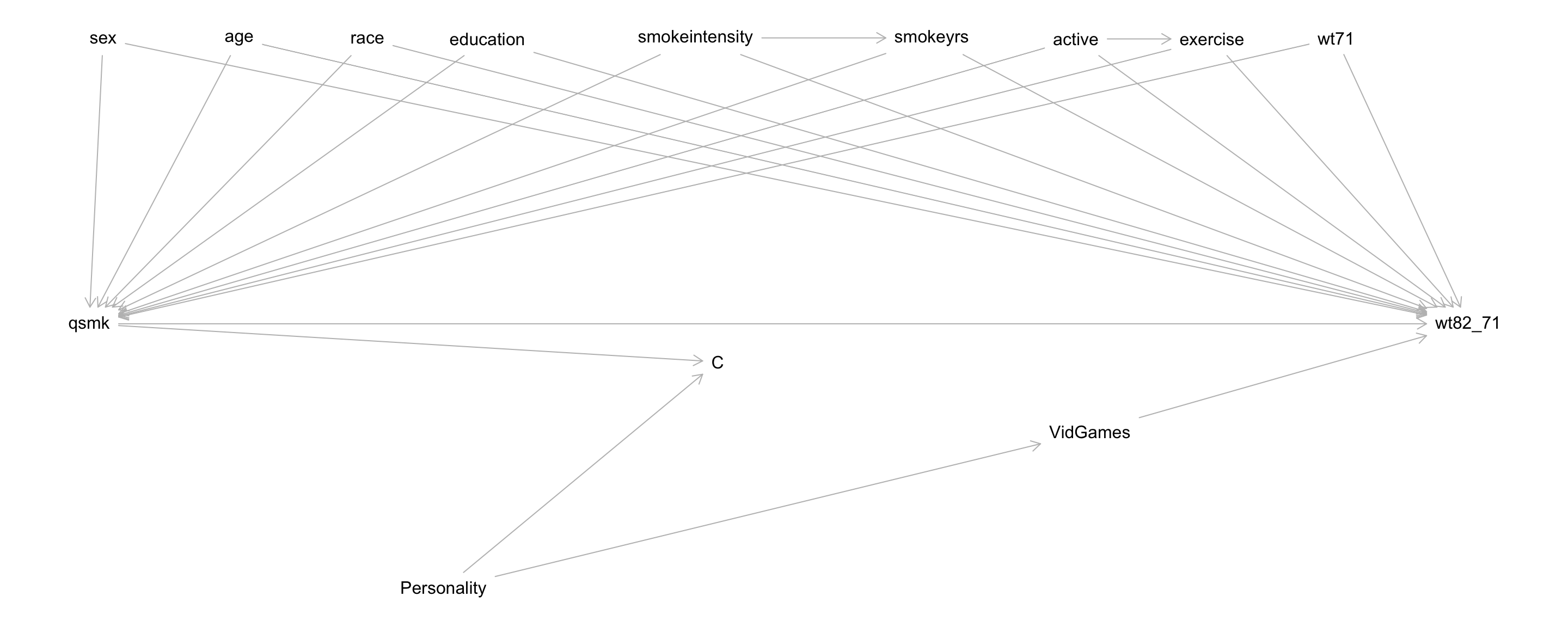
- e.g., The DAG below. View \(C\) as the new “treatment” variable.
- Another way to put it: when we put a box around \(C\) in the DAG, \(Z\) must d-separate \(A\) and \(Y\) under the null.
  Same condition as before, now explicit about paths with conditioned-on colliders (non-backdoor paths).

Questions: \(C\) is inherently conditioned on in our analysis (\(C = 0\)).

What set \(Z\) d-separates the treatment and outcome under the null?
What is a set \(Z_2\) such that \(Z_2 \cup A\) (read \(Z_2\) “union” \(A\), or \(Z_2\) and \(A\) together) d-separate \(C\) and the outcome?

Conclusion:

\(Z\) should include:
sex, age, race, education, smokeintensity, smokeyrs, active, exercise, wt71, and VidGames
(Same as before with the addition of VidGames)
\(Z\) blocks spurious, non-causal paths between \(A\) (qsmk) and \(Y\) (wt82_71)

\(Z_2\) should include VidGames
Together with \(A\), \(Z_2\) blocks spurious, non-causal paths between \(C\) and \(Y\)
Note that \(Z_2\) is contained within \(Z\).
- This will be the case when \(A\) is a cause of \(C\) (often true).

Ultimate goal: Want to upweight individuals using \(P(A, C = 0 \mid Z)\)

Why? Same rationale as our tree diagram with additional \(C = 1\) and \(C = 0\) branches.
Allows us to estimate \(E[Y^{a, c = 0}]\): expected potential outcome under treatment \(a\) and when no one has been censored (\(C = 0\))

We can express \(P(A, C = 0 \mid Z)\) as the following:

\[ \begin{align*} P(A, C = 0 \mid Z) &= P(A, C = 0, Z)/P(Z) \\ &= P(A \mid Z) P(C = 0 \mid A, Z) \end{align*} \]

Based on the last line, we see (1) the propensity score and (2) another “propensity” of being uncensored.
Will want models for both.
(The censoring probability is not typically called a propensity score.)

A little extra theory (don’t worry about the math part below if you haven’t taken Probability):

\(Z\) may contain extra variables not in \(Z_2\) if there are, say, many common causes of \(A\) and \(Y\), but only a few of these are a cause of \(C\). Let’s say that these extra variables are in the set \(Z_1\). (\(Z = Z_1 \cup Z_2\))

If the variables in \(Z_1\) are not causes of \(C\), then \(C\) and \(Z_1\) are conditionally independent given \(A\) and \(Z_2\).

Going through the work below…

\[ \begin{align*} P(A, C = 0 \mid Z) &= P(A, C = 0 \mid Z_1, Z_2) \\ &= P(A, C = 0, Z_1, Z_2)/P(Z_1, Z_2) \\ &= P(A \mid Z_1, Z_2) P(C = 0 \mid A, Z_1, Z_2) \\ &= P(A \mid Z_1, Z_2) P(C = 0 \mid A, Z_2) \end{align*} \]

…this implies that the propensity score model (for \(A\)) should depend on all variables in \(Z\) (the set \(Z_1\) and \(Z_2\) together) and that the censoring probability model only need depend on \(Z_2\).

Analysis plan:

Notation:

\(Z\) is the set that d-separates \(A\) and \(Y\) when \(C\) is conditioned on.
\(Z_2\) (a subset of \(Z\)) that, together with \(A\), d-separates \(C\) and \(Y\)

Model the propensity scores \(P(A\mid Z)\) using all variables \(Z\) in the d-separating set. Create inverse probability weights \(W^A = 1/P(A\mid Z)\) (treatment weights).
Model the probability of censoring \(P(C \mid A, Z_2)\). Create inverse probability weights \(W^C = 1/P(C = 0\mid A, Z_2)\) (censoring weights).
Create final weights (for treatment and censoring) \(W^{A,C} = W^A\times W^C\).
Fit the desired marginal structural model with these final weights.

Exercises

A template Rmd is available here.

Setup

library(readr)
library(dplyr)
library(ggplot2)
library(geepack)

nhefs <- read_csv("https://cdn1.sph.harvard.edu/wp-content/uploads/sites/1268/1268/20/nhefs.csv")

Create a censoring indicator variable that will be TRUE if the individual was censored and FALSE otherwise.

nhefs$cens <- is.na(nhefs$wt82_71)

Throughout we’ll use the full nhefs dataset, and we’ll work from the DAG below (\(C\) has been conditioned on):

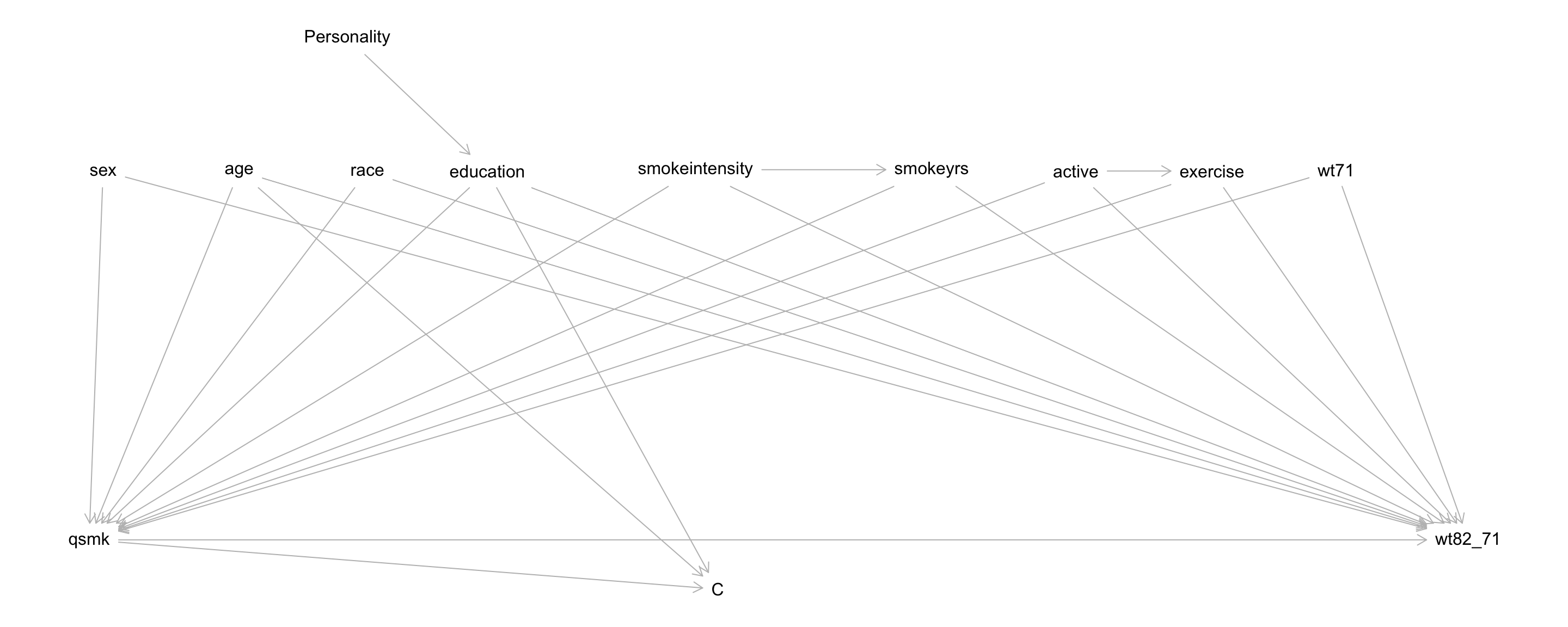
Part 1: Modeling to obtain weights

Based on the DAG above, identify the set of variables \(Z\) that d-separates qsmk and weight gain.
Fit an appropriate treatment propensity score model, and call this ps_treat_mod. For simplicity, assume that a quadratic relationship for the quantitative variables gives a good fit. Make sure to wrap categorical variables inside factor() in your model formula.
Add a new variable to your dataset called weights_treat that contains the IP weights for treatment.

Is it believable that quitting smoking (treatment) is a cause of censoring? How do the tabulations/calculations below help answer this?

# P(censored | quitters) and P(censored | nonquitter)
table(qsmk = nhefs$qsmk, cens = nhefs$cens)
table(qsmk = nhefs$qsmk, cens = nhefs$cens) %>% prop.table(margin = 1)

How would you see if the data support the age --> C and education --> C arrows? Describe, but don’t actually perform this analysis.
Fit an appropriate model for the probability of censoring, and call this prob_cens_mod. For simplicity, assume that a quadratic relationship for the quantitative variables gives a good fit. Make sure to wrap categorical variables inside factor() in your model formula.
Add a new variable to your dataset called weights_cens that contains the IP weights for censoring. (Note that in R, the default for logistic regression is to model the probability of the outcome variable equaling 1.)
Add a final weight variable to your dataset called weight_TC.

Part 2: Fitting MSMs

Fit the following two MSMs (\(A\) is qsmk, and for sex, 0 indicates males and 1 indicates females):

\[ E[Y^{a, c=0}] = \beta_0 + \beta_1 a \] \[ E[Y^{a, c=0}] = \beta_0 + \beta_1 a + \beta_2\hbox{sex} + \beta_3 a\times\hbox{sex} \]

Note: In our previous analysis where we worked with nhefs_subs, we had actually fit the following:

\[ E[Y^{a} \mid C = 0] = \beta_0 + \beta_1 a \] \[ E[Y^{a} \mid C = 0] = \beta_0 + \beta_1 a + \beta_2\hbox{sex} + \beta_3 a\times\hbox{sex} \]

Refit these models here using the relevant weights. How do your results compare?