Topic 12 IPW: Simulation

Learning Goals

Use simulation to understand the importance of correct model specification on the performance of IPW and to verify the “arrow-removing” property of IPW

Slides from today are available here.

Exercises

You can download a template RMarkdown file to start from here.

Exercise 1: Simulate

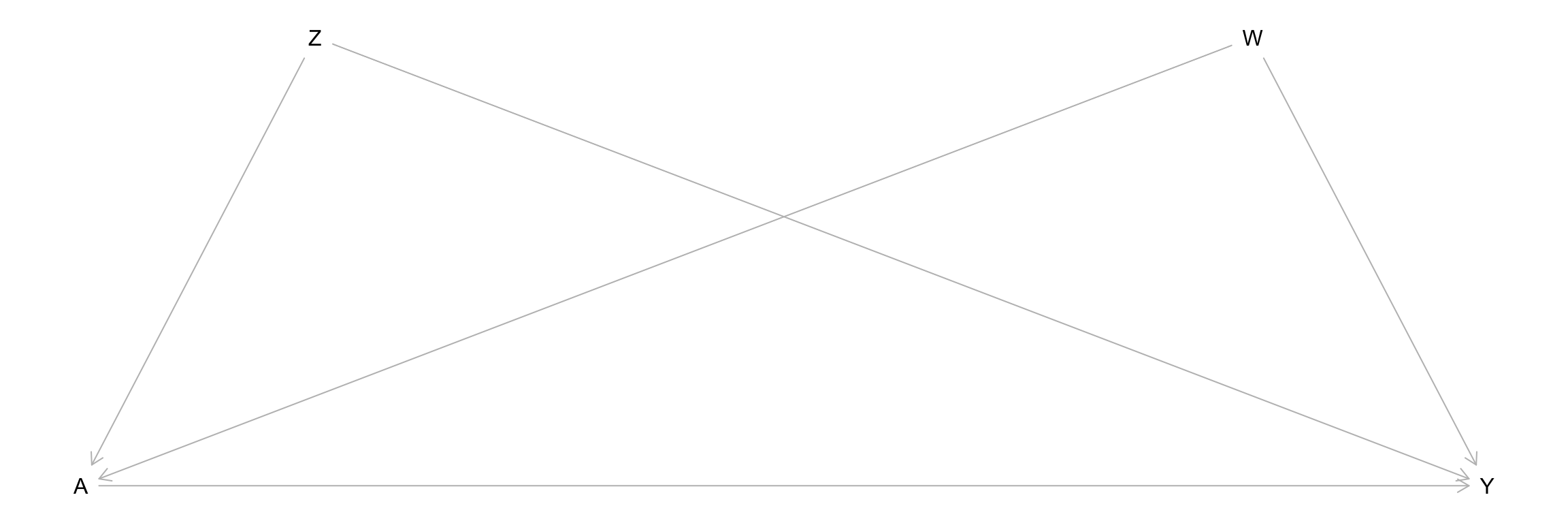
We’ll simulate data from the causal graph below where \(Z\), \(W\), and \(A\) are binary, and \(Y\) is quantitative. Use the structural equations below for \(A\) and \(Y\), and store your simulated data as sim_data.

\(\log(\mathrm{odds}(A = 1)) = -1 + 0.4 Z + 0.4 W + 0.9 Z*W\)
\(Y\) follows a normal distribution with mean \(10 + 5A + 6Z + 7W\) and standard deviation 2.

Based on the structural equation for \(Y\), what is the true ACE? Based on the causal graph, what variables are needed to achieve conditional exchangeability?

set.seed(451)
n <- 10000
Z <- rbinom(n, size = 1, prob = 0.5)
W <- rbinom(n, size = 1, prob = 0.5)

log_odds_A <- 
odds_A <- 
p_A <- 
A <- 

noise_Y <- rnorm(___)
mean_Y <- 
Y <- mean_Y + noise_Y

sim_data <- data.frame(Z = factor(Z), W = factor(W), A = factor(A), Y)

Exercise 2: Inverse probability weighting

Here, we’ll check the performance of inverse probability weighting for estimating the average causal effect.

The accuracy of IPW depends on having the right model for treatment as a function of the variables needed to achieve conditional exchangeability.
- Based on our simulation, what is the correct logistic regression model that should be fit? Fit this model as ps_mod_complex.
- Also fit a wrong model called ps_mod_simple that uses the formula A ~ Z + W. (In this way, we can explore the impact of model misspecification.)

The code below uses your models to compute (right and wrong) IP weights.

predict(logistic_mod, newdata = data_to_make_predictions_for, type = "response") is used to predict probabilities from a logistic regression model. (Without type = "response", log-odds are computed.)
Add comments to this code to document these different pieces, and check in with the instructor if you have questions.

sim_data <- sim_data %>%
    mutate(
        ps_simple = predict(ps_mod_simple, newdata = sim_data, type = "response"),
        ipw_simple = case_when(
            A==1 ~ 1/ps_simple,
            A==0 ~ 1/(1-ps_simple)
        )
    ) %>%
    mutate(
        ps_complex = predict(ps_mod_complex, newdata = sim_data, type = "response"),
        ipw_complex = case_when(
            A==1 ~ 1/ps_complex,
            A==0 ~ 1/(1-ps_complex)
        )
    )

Fit an ordinary regression model Y ~ A that ignores the IP weights. Is the estimated ACE what you expected?
Incorporate the IP weights into your analysis by modifying your model from part c as below. (As discussed in 12.4 of WHATIF, this weighting fits a marginal structural model (MSM) that allows us to directly estimate the ACE.) Is the estimated ACE what you expected?
```
lm(..., data = ..., weights = ipw_simple)
lm(..., data = ..., weights = ipw_complex)
```

Note: Using weights = ... in glm(..., family = "binomial") does not work exactly the way we want it to. (It works as we want for lm().) Going forward, we will use a specialized package (the survey package) for dealing with weights.

Exercise 3: Balance checking

What is the key differentiator between regression and inverse probability weighting?
Let’s verify that unique property of IP weighting. Make plots to show the relationship between \(Z\) and \(A\) and between \(W\) and \(A\) in the original, unweighted data.
Modify your plot to incorporate the IP weights by adding the following to aes(). What property of IP weighting does this show?
```
aes(..., weight = ipw_complex)
```