Introduction to multiple regression

Notes and in-class exercises

Notes

You can download a template file to work with here.
File organization: Save this file in the “Activities” subfolder of your “STAT155” folder.

Learning goals

By the end of this lesson, you should be familiar with:

some limitations of simple linear regression
the general goals behind multiple linear regression
strategies for visualizing and interpreting multiple linear regression models of \(y\) vs 2 predictors, 1 quantitative and 1 categorical

Readings and videos

Today is a day to discover ideas, so no readings or videos to go through before class.

Motivation

EXAMPLE 1

Let’s explore some data on penguins.

First, enter install.packages("palmerpenguins") in the console (not Rmd).

Then load the penguins data.

You can find a codebook for these data by typing ?penguins in your console (not Rmd).

# Load packages
library(readr)
library(ggplot2)
library(dplyr)

# Load data
library(palmerpenguins)
data(penguins)
penguins <- penguins %>% 
    filter(species != "Adelie", bill_length_mm < 57)

# Check it out
head(penguins)

# A tibble: 6 × 8
  species island bill_length_mm bill_depth_mm flipper_length_mm body_mass_g
  <fct>   <fct>           <dbl>         <dbl>             <int>       <int>
1 Gentoo  Biscoe           46.1          13.2               211        4500
2 Gentoo  Biscoe           50            16.3               230        5700
3 Gentoo  Biscoe           48.7          14.1               210        4450
4 Gentoo  Biscoe           50            15.2               218        5700
5 Gentoo  Biscoe           47.6          14.5               215        5400
6 Gentoo  Biscoe           46.5          13.5               210        4550
# ℹ 2 more variables: sex <fct>, year <int>

Our goal is to build a model that we can use to get good predictions of penguins’ flipper (“arm”) lengths.

Consider 2 simple linear regression models of flipper_length_mm by penguin sex and species:

summary(lm(flipper_length_mm ~ sex, penguins))$r.squared

[1] 0.1204716

summary(lm(flipper_length_mm ~ species, penguins))$r.squared

[1] 0.7013577

How might we improve our predictions of flipper_length_mm using only these 2 predictors?

What do you think our new R-squared would be?

EXAMPLE 2

Consider a simple linear regression model of flipper_length_mm by bill_length_mm:

penguins %>% 
    ggplot(aes(y = flipper_length_mm, x = bill_length_mm)) + 
    geom_point() + 
    geom_smooth(method = "lm", se = FALSE)

`geom_smooth()` using formula = 'y ~ x'

Thoughts? What’s going on here?

How does this highlight the limitations of a simple linear regression model?

EXAMPLE 3

The cps dataset contains employment information collected by the U.S. Current Population Survey (CPS) in 2018.

We can use these data to explore wages among 18-34 year olds.

The original codebook is here.

# Import data
cps <- read_csv("https://mac-stat.github.io/data/cps_2018.csv") %>% 
    select(-education, -hours) %>% 
    filter(age >= 18, age <= 34) %>% 
    filter(wage < 250000)

Rows: 10000 Columns: 8
── Column specification ────────────────────────────────────────────────────────
Delimiter: ","
chr (4): marital, industry, health, education_level
dbl (4): wage, age, education, hours

ℹ Use `spec()` to retrieve the full column specification for this data.
ℹ Specify the column types or set `show_col_types = FALSE` to quiet this message.

# Check it out
head(cps)

# A tibble: 6 × 6
   wage   age marital industry   health    education_level
  <dbl> <dbl> <chr>   <chr>      <chr>     <chr>          
1 75000    33 single  management fair      bachelors      
2 33000    19 single  management very_good bachelors      
3 43000    33 married management good      bachelors      
4 50000    32 single  management excellent HS             
5 14400    28 single  service    excellent HS             
6 33000    31 married management very_good bachelors

We can use a simple linear regression model to summarize the relationship of wage with marital status:

# Build the model
wage_mod <- lm(wage ~ marital, data = cps)

# Summarize the model
coef(summary(wage_mod))

               Estimate Std. Error   t value     Pr(>|t|)
(Intercept)    46145.23    921.062  50.10002 0.000000e+00
maritalsingle -17052.37   1127.177 -15.12839 5.636068e-50

What do you / don’t you conclude from this model?

How does it highlight the limitations of a simple linear regression model?

Reflection: Why are multiple regression models so useful?

We can put more than 1 predictor into a regression model! Adding predictors to models…

Predictive viewpoint: Helps us better predict the response
Descriptive viewpoint: Helps us better understand the isolated (causal) effect of a variable by holding constant confounders

Multiple linear regression model formula

In general, a multiple linear regression model of \(y\) with multiple predictors \((x_1, x_2, ..., x_p)\) is represented by the following formula:

\[E[y \mid x_1, x_2, ..., x_p] = \beta_0 + \beta_1 x_1 + \beta_2 x_2 + ... + \beta_p x_p\]

Exercises

In the coming weeks, we’ll explore how to visualize, interpret, build, and evaluate multiple linear regression models.

First, we’ll explore some foundations using a model of penguin flipper_length_mm by just 2 predictors: bill_length_mm (quantitative) and species (categorical).

Exercise 1: Visualizing the relationship

We’ve learned how to visualize the relationship of flipper_length_mm by bill_length_mm alone:

penguins %>% 
    ggplot(aes(y = flipper_length_mm, x = bill_length_mm)) + 
    geom_point()

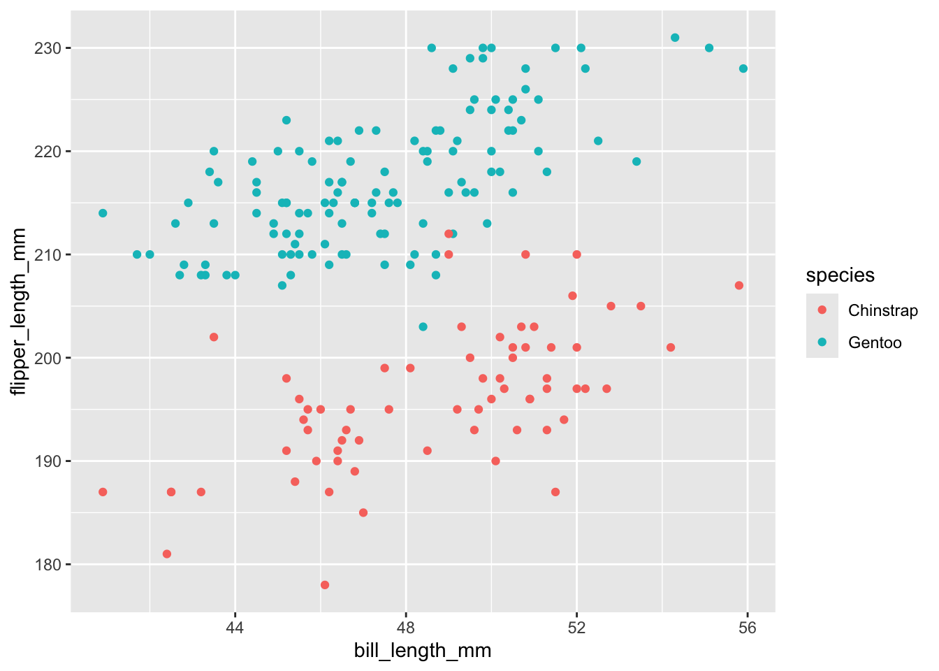
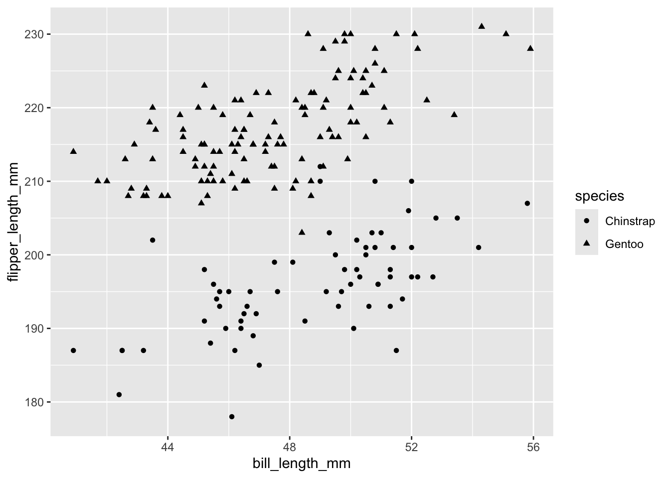
THINK: How might we change the scatterplot points to also indicate information about penguin species? (There’s more than 1 approach!)
Try out your idea by modifying the code below. If you get stuck, talk with the tables around you!

penguins %>%
    ggplot(aes(y = flipper_length_mm, x = bill_length_mm, ___ = ___)) +
    geom_point()

Exercise 2: Visualizing the model

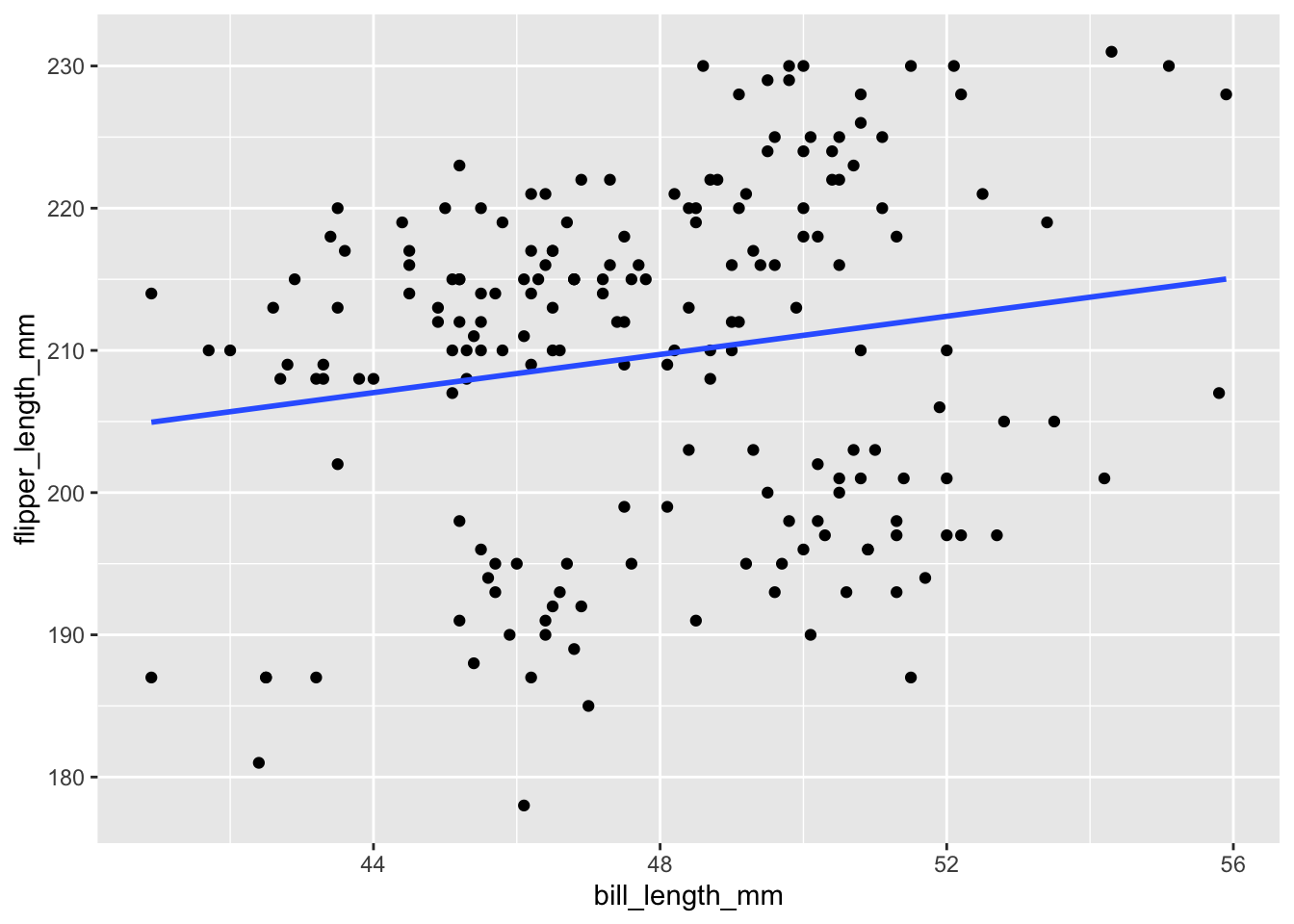
We’ve also learned that a simple linear regression model of flipper_length_mm by bill_length_mm alone can be represented by a line:

penguins %>% 
    ggplot(aes(y = flipper_length_mm, x = bill_length_mm)) + 
    geom_point() + 
    geom_smooth(method = "lm", se = FALSE)

THINK: Reflecting on your plot of flipper_length_mm by bill_length_mm and species in Exercise 1, how do you think a multiple regression model of flipper_length_mm using both of these predictors would be represented?
Check your intuition below by modifying the code below to include species in this plot, as you did in Exercise 1.

penguins %>%
    ggplot(aes(y = flipper_length_mm, x = bill_length_mm, ___ = ___)) +
    geom_point() +
    geom_smooth(method = "lm", se = FALSE)

Exercise 3: Intuition

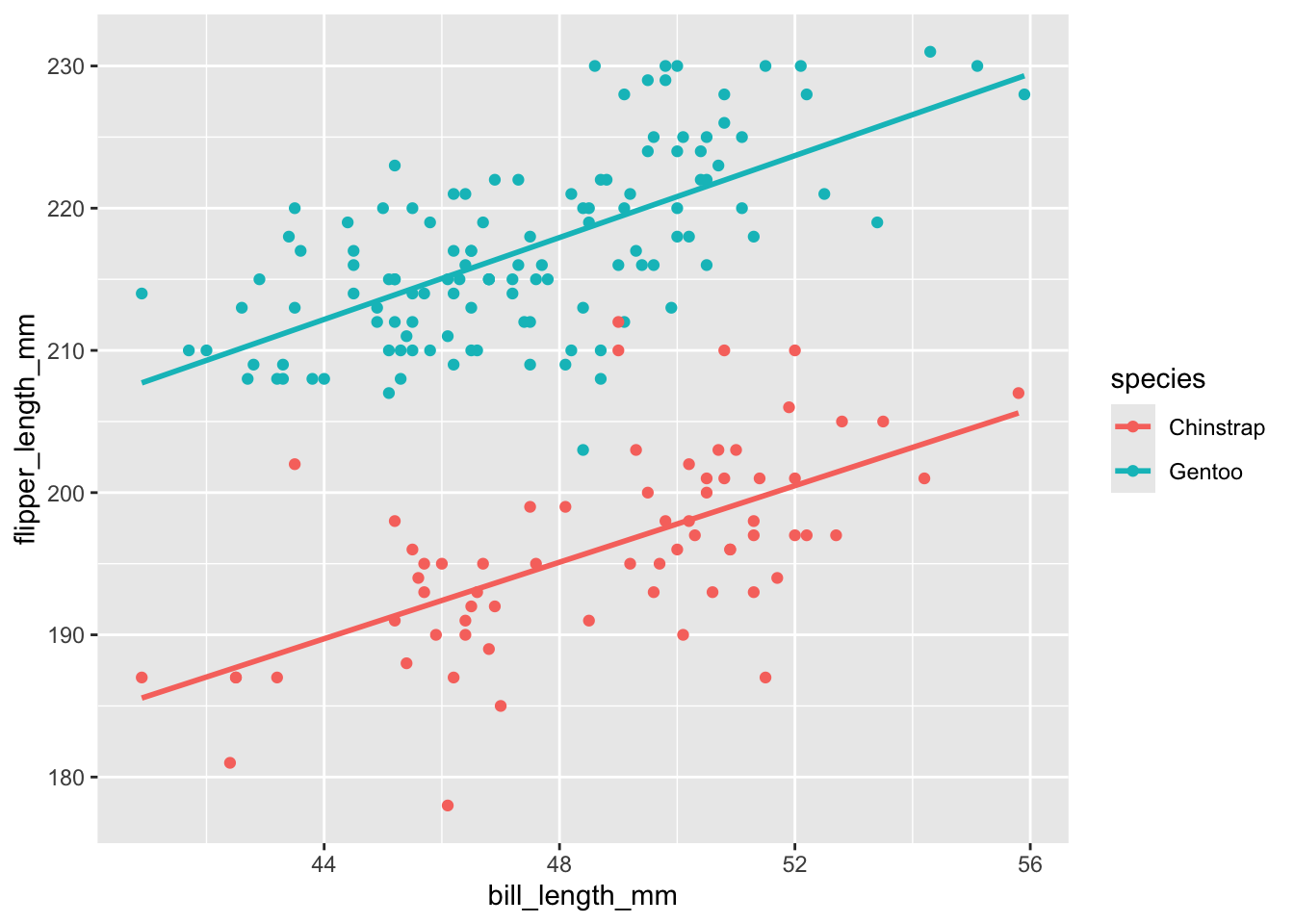
Your plot in Exercise 2 demonstrated that the multiple linear regression model of flipper_length_mm by bill_length_mm and species is represented by 2 lines.

Let’s interpret those lines!

For each question, provide an answer along with evidence from the model lines that supports your answer.

What’s the relationship between flipper_length_mm and species, no matter a penguin’s bill_length_mm?
What’s the relationship between flipper_length_mm and bill_length_mm, no matter a penguin’s species?
Does the rate of increase in flipper_length_mm with bill_length_mm differ between the two species?

Exercise 4: Model formula

Of course, there’s a formula behind the multiple regression model.

We can obtain this using the usual lm() function.

# Build the model
penguin_mod <- lm(flipper_length_mm ~ bill_length_mm + species, data = penguins)

# Summarize the model
coef(summary(penguin_mod))

In the lm() function, how did we communicate that we wanted to model flipper_length_mm by both bill_length_mm and species?
Complete the following model formula:

E[flipper_length_mm | bill_length_mm, speciesGentoo] = ___ + ___ * bill_length_mm + ___ * speciesGentoo

Exercise 5: Sub-model formulas

Ok. We now have a single formula for the model.

And we observed earlier that this formula is represented by two lines: one describing the relationship between flipper_length_mm and bill_length_mm for Chinstrap penguins and the other for Gentoo penguins.

Let’s bring these ideas together.

Utilize the model formula to obtain the equations of these two lines, i.e. to obtain the sub-model formulas for the 2 species. Hint: Plug speciesGentoo = 0 and speciesGentoo = 1.

Chinstrap: flipper_length_mm = ___ + ___ bill_length_mm

Gentoo: flipper_length_mm = ___ + ___ bill_length_mm

Exercise 6: coefficients – physical interpretation

Reflecting on Exercise 5, let’s interpret what the model coefficients tell us about the physical properties of the two 2 sub-model lines. Choose the correct option given in parentheses:

The intercept coefficient, 127.75, is the intercept of the line for (Chinstrap / Gentoo) penguins.
The bill_length_mm coefficient, 1.40, is the (intercept / slope) of both lines.
The speciesGentoo coefficient, 22.85, indicates that the (intercept / slope) of the line for Gentoo is 22.85mm higher than the (intercept / slope) of the line for Chinstrap. Similarly, since the lines are parallel, the line for Gentoo is 22.85mm higher than the line for Chinstrap at any bill_length_mm.

Exercise 7: coefficients – contextual interpretation

Next, interpret each coefficient in a contextually meaningful way. What do they tell us about penguin flipper lengths?!

Interpret 127.75 (intercept of the Chinstrap line).
Interpret 1.40 (slope of both lines). For both Chinstrap and Gentoo penguins, we expect…
Interpret 22.85. At any bill_length_mm, we expect…

Exercise 8: Prediction

Now that we better understand the model, let’s use it to predict flipper lengths!

Recall the model summary and visualization:

coef(summary(penguin_mod))

penguins %>% 
    ggplot(aes(y = flipper_length_mm, x = bill_length_mm, color = species)) + 
    geom_point() + 
    geom_smooth(method = "lm", se = FALSE)

Predict the flipper length of a Chinstrap penguin with a 50mm long bill. Make sure your calculation is consistent with the plot.

127.75 + 1.40*___ + 22.85*___

Predict the flipper length of a Gentoo penguin with a 50mm long bill. Make sure your calculation is consistent with the plot.

127.75 + 1.40*___ + 22.85*___

Use the predict() function to confirm your predictions in parts a and b.

# Confirm the calculation in part a
predict(penguin_mod,
        newdata = data.frame(bill_length_mm = ___, species = "___"))

# Confirm the calculation in part b
predict(penguin_mod,
        newdata = data.frame(bill_length_mm = ___, species = "___"))

Exercise 9: R-squared

Finally, recall that improving our predictions was one motivation for multiple linear regression (using 2 predictors instead of 1).

To this end, consider the R-squared values of the simple linear regression models that use just one predictor at a time:

summary(lm(flipper_length_mm ~ bill_length_mm, data = penguins))$r.squared

summary(lm(flipper_length_mm ~ species, data = penguins))$r.squared

If you had to use only 1 of our 2 predictors, which would give the better predictions of flipper_length_mm?
What do you guess is the R-squared of our multiple regression model that uses both of these predictors? Why?
Check your intuition. How does the R-squared of our multiple regression model compare to that of the 2 separate simple linear regression models?

summary(penguin_mod)$r.squared

Reflection

You’ve now explored your first multiple regression model! Thus you likely have a lot of questions about what’s to come. What are they?

Response: Put your response here.

Solutions