Topic 11 Inverse Probability Weighting

Pre-class work

Videos/slides

Estimating Causal Effects: Inverse Probability Weighting: [video], [slides]

Checkpoint

Learning Goals

Verify properties of inverse probability weighting for estimating average causal effects using simulation

Exercises

Solutions to these exercises are available on Moodle.

Navigate to PollEverywhere for some warm-up exercises.

You can download a template RMarkdown file to start from here.

Exercise 1: Simulate

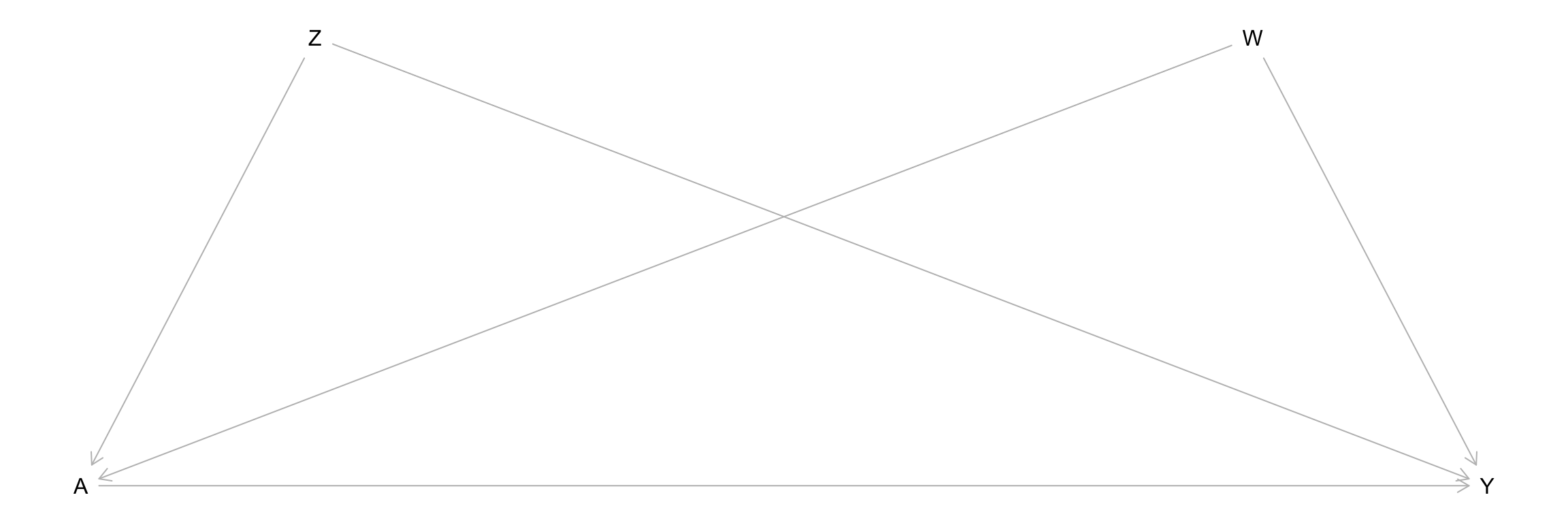
Simulate data from the causal graph below where \(Z\), \(W\), and \(A\) are binary, and \(Y\) is quantitative. Use the model below for your structural equation for \(A\), and store your data in a dataset object called sim_data.

\[ \log(\mathrm{odds}(A = 1)) = -1 + 0.4 Z + 0.4 W + 0.9 Z*W \]

Exercise 2: Intervene

Based on your SEM, what do you expect to be the average causal effect? Modify your simulation to simulate an intervention where all are treated and all are untreated to verify that this is the true average causal effect.

Exercise 3: Inverse probability weighting

Here, we’ll check the performance of inverse probability weighting for estimating the average causal effect.

In practice, we don’t know the true SEM underlying the data, so we need to estimate the appropriate weights from the data. This starts from estimating the probability of receiving treatment conditional on appropriate variables. (This probability is called the propensity score.) Fit an appropriate propensity score model called ps_mod.
The code below uses your fitted ps_mod to compute IP weights.
- Look up the mutate() and case_when() functions from dplyr by entering ?function_name in the Console.
- predict(logistic_mod, newdata = data_to_make_predictions_for, type = "response") is used to predict probabilities from a logistic regression model. (Without type = "response", log-odds are computed.)
- Add comments to this code to document these different pieces, and check in with the instructor if you have questions.
```
sim_data <- sim_data %>%
    mutate(
        ps = predict(ps_mod, newdata = sim_data, type = "response"),
        ip_weight = case_when(
            A==1 ~ 1/ps,
            A==0 ~ 1/(1-ps)
        )
    )
```
Fit an ordinary regression model Y ~ A that ignores the IP weights. Is the estimated ACE what you expected?
Incorporate the IP weights into your analysis by modifying your model from part c as below. Is the estimated ACE what you expected?
```
lm(..., data = ..., weights = ip_weight)
```

Note: Using weights = ... in glm(..., family = "binomial") does not work exactly the way we want it to. (It works as we want for lm().) Going forward, we will use a specialized package (the survey package) for dealing with weights.

Exercise 4: Balance checking

What is the key differentiator between regression and inverse probability weighting?
Let’s verify that unique property of IP weighting. Make plots to show the relationship between \(Z\) and \(A\) and between \(W\) and \(A\) in the original, unweighted data.
Modify your plot to incorporate the IP weights by adding the following to aes(). What property of IP weighting does this show?
```
aes(..., weight = ip_weight)
```

Extra!

If you’ve taken Statistical Machine Learning, what connections can you make between ideas about predictive modeling and propensity score estimation? If you haven’t taken that course but are curious, feel free to ask the instructor!

Take a few minutes to reflect on today’s ideas by filling out an exit ticket.