Topic 1 Review and Motivation
Learning Goals
- Identify when linear regression and when logistic regression would be appropriate
- Interpret coefficients from linear and logistic regression models with and without interaction
- Describe the 2 conditions/characteristics of a confounder
- Use a causal diagram (a graph) to depict the structure of relationships underlying confounding
- Explain how regression models provide a way to “adjust for” confounders
- Using the 2 characteristics of a confounder, explain how an “unadjusted” relationship is misleading
Exercises
You can download a template RMarkdown file to start from here.
We will look at (simulated) data from a study that looked at the effectiveness of chemotherapy for treating colon cancer. Chemotherapy is effectively a poison that kills cells in the body that are rapidly proliferating: these cells include the cancer cells (often in a mass called a tumor) but also cells in bone marrow involved in sustaining the immune system.
In this study, researchers measured the following variables:
pre_tumor_size: Tumor size at the start of the study (SmallorLarge).treated:ChemoYesif the patient received chemotherapy orChemoNoif not.post_tumor_size: Tumor size 3 months after the start of the study (SmallorLarge).recovery:Yesif the patient fully recovered from their cancer after 1 year.Nootherwise.
You can read in the data as follows:
chemo_study_data <- readr::read_csv("https://www.dropbox.com/s/vl06j75a8afw8ct/chemo_study.csv?dl=1")Exercise 1: Plots and confounders
The first step in any data analysis is to visualize your data. Let’s refamiliarize ourselves with the ggplot2 package in R. It may be helpful to have this ggplot2 cheat sheet open. Make sure to load the ggplot2 package by including library(ggplot2) at the top of your RMarkdown document.
- Get a feel for the data by visualizing the distributions of all 4 variables individually (4 plots total). Your code should look something like below.
ggplot(chemo_study_data, aes(x = pre_tumor_size)) + ???- Is pre-treatment tumor size predictive of whether or not a patient received chemotherapy? Make a plot to assess this, and briefly state what conclusions can be drawn from the plot. (Hint: it will be helpful to look at the second page of the cheat sheet in the section labeled “Position Adjustments”.)
ggplot(chemo_study_data, aes(x = pre_tumor_size, fill = treated)) + ???- Is pre-treatment tumor size predictive of whether or not a patient recovered? Make a plot, and briefly state your conclusions.
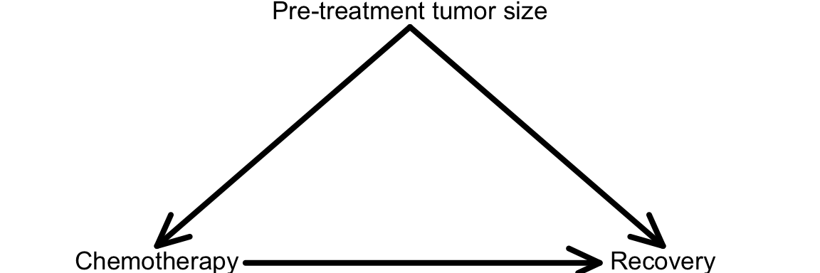
- A variable is a confounder if it is a common cause of both the treatment and outcome. This is shown in the diagram below. Given your results from parts b and c, could pre-treatment tumor size be a confounder of the relationship between chemotherapy treatment and recovery?
- Could post-treatment tumor size be a confounder of the relationship between chemotherapy treatment and recovery? Support your answer with plots and an explanation.
Note: the causal relationships of interest so far can be depicted in a causal diagram, shown below. An arrow between two variables indicates that one is a cause of the other (an arrow points from a cause to its effect).
Exercise 2: Implications of confounding
- What is the relationship between confounders and the saying “Correlation does not imply causation”?
- Explain how regression models can be used to remove the influence of confounding variables.
- Suppose that chemotherapy generally works to promote recovery. Suppose also that sicker patients tend to receive chemotherapy, and healthier patients tend to not receive chemotherapy. What would you expect if you directly compared recovery rates in the chemotherapy and standard of care patients (no adjustments for other variables)? What would you expect if you held appropriate confounders constant?
Exercise 3: Logistic regression models
We can model recovery using a logistic regression model (used when the outcome variable is binary). In R, we can fit a logistic regression model using code like the following:
# Fit the model and store it in the "mod" object
mod <- glm(outcome_variable ~ predictor_variable1+predictor_variable2,
    family = "binomial", data = your_data)

# Display model output
summary(mod)

# Obtain confidence intervals (CIs) for model coefficients
# (95% CIs by default)
confint(mod)- Fit a logistic regression model with only treatment as a predictor. Interpret the treatment coefficient. Is the sign of the coefficient what you expected? Why is this model misleading?
- Fit a logistic regression model that adjusts for pre-treatment tumor size. Interpret the treatment coefficient. Is the sign of the coefficient what you expected? Also report the 95% confidence interval for the treatment coefficient and what information you learn from it. (Side note: This article by Eleanor Murray has a great explanation of the most common misinterpretation of confidence intervals.)
- Fit a logistic regression model that adjusts for pre- and post-treatment tumor size. Interpret the treatment coefficient. Is the sign of the coefficient what you expected?
Exercise 4: Warming up to causal ideas
- Consider the statement: “The causal effect of chemotherapy on recovery rates (as compared to no chemotherapy) is a change (difference) of 10%.” What do you think “causal effect” means? What would you like it to mean?
- Which model do you think best estimates the causal effect of chemotherapy on recovery rates? Explain.