Topic 18 Bagging and Random Forests (Coding)
Exercises
You can download a template RMarkdown file to start from here.
Before proceeding, install the ranger and vip packages.
Our goal will be to classify types of urban land cover in small subregions within a high resolution aerial image of a land region. Data from the UCI Machine Learning Repository include the observed type of land cover (determined by human eye) and “spectral, size, shape, and texture information” computed from the image. See this page for the data codebook.
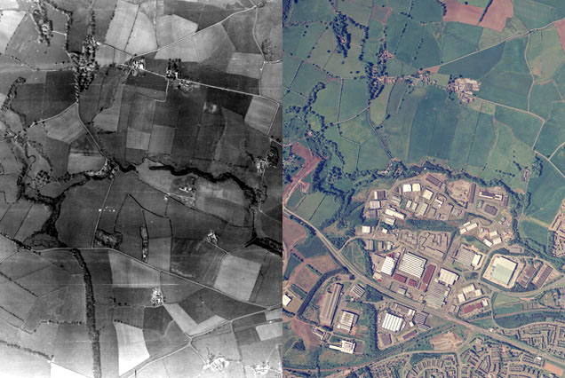
Source: https://ncap.org.uk/sites/default/files/EK_land_use_0.jpg
library(dplyr)
library(readr)
library(ggplot2)
library(tidymodels)
tidymodels_prefer()


# Read in the data
land <- read_csv("https://www.dropbox.com/s/r59esfepjw7qsg0/land_cover_training.csv?dl=1")

# There are 9 land types, but we'll focus on 3 of them
land <- land %>%
    filter(class %in% c("asphalt", "grass", "tree")) %>%
    mutate(class = factor(class))
Exercise 1: Building a random forest in tidymodels
If you want to use the land dataset, the code is complete, but you should step through to understand what each line is doing.
If you are using your project dataset, you don’t need to do anything here if you finished implementing a random forest from last class.
set.seed(123)

# Model Specification
rf_spec <- rand_forest() %>%
    set_engine(engine = "ranger") %>%
    set_args(
        mtry = NULL, # size of random subset of variables; default is floor(sqrt(number of total predictors))
        trees = 1000, # Number of trees
        min_n = 2,
        probability = FALSE, # FALSE: get hard predictions (not needed for regression)
        importance = "impurity"
    ) %>%
    set_mode("classification") # change this for regression

# Recipe
data_rec <- recipe(class ~ ., data = land)

# Workflows
data_wf <- workflow() %>%
    add_model(rf_spec) %>%
    add_recipe(data_rec)

# Note how we're not using tune_grid() or vfold_cv() information here
rf_fit <- fit(data_wf, data = land)
Exercise 2: Evaluate model performance
Printing the rf_fit object displays information about the random forest model.
Report and interpret the OOB prediction error value in the context of your data. (Misclassification rate is reported for classification, and MSE is reported for regression.)
rf_fitClassification
We can look at a confusion matrix resulting from the out-of-bag (OOB) predictions.
- Check your conceptual understanding: How are OOB predictions made?
- Based on the confusion matrix, what classes are predicted most accurately, and does this make sense contextually?
rf_output <- land %>%
    mutate(OOB_pred_class = rf_fit %>% extract_fit_engine() %>% pluck("predictions")) # This extracts the OOB predictions

conf_mat(
    data = rf_output,
    truth = class,
    estimate = OOB_pred_class
)
We can also explore how misclassification rates relate to predictors. The code below creates a new variable is_misclass indicating whether or not a case was misclassified in the OOB predictions.
- Make visualizations of
is_misclassand each of your predictors individually to explore how misclassification rate might vary across predictors.
rf_output <- rf_output %>%
    mutate(is_misclass = class!=OOB_pred_class)
Regression
We can compute residuals resulting from OOB predictions.
- Check your conceptual understanding: How are OOB predictions made?
- Make residual plots to visualize how errors might relate to your predictors.
rf_output <- land %>%
    mutate(
        OOB_pred = rf_fit %>% extract_fit_engine() %>% pluck("predictions"),  # This extracts the OOB predictions
        resid = YOUR_OUTCOME - OOB_pred
    )

# Residual plots vs individual predictors
Exercise 3: Variable importance
(You’ll need to install the vip package before proceeding.)
Because bagging and random forests use many trees, the nice interpretability of single decision trees is lost. However, we can still get a measure of how important the different predictors were in this predicting the outcome.
For each of the predictors, the code below gives the “total decrease in node impurities from splitting on the variable, averaged over all trees” (package documentation).
- Do the variable importance results make sense contextually? (If you’re using the
landdataset, check out the codebook for these variables here.) - Conceptual question: It has been found that measures of variable importance from random forests can tend to favor predictors with a lot of unique values. Explain briefly why this makes sense by thinking about the recursive binary splitting algorithm for a single tree. (Note: similar cautions arise for variable importance in single trees.)
library(vip)

# Plot of the variable importance information
rf_fit %>%
    extract_fit_engine() %>%
    vip(num_features = 30) + theme_classic()

# Extract the numerical information on variable importance and display the most and least important predictors
rf_var_imp <- rf_fit %>%
    extract_fit_engine() %>%
    vip::vi()
head(rf_var_imp)
tail(rf_var_imp)