Topic 11 Trees (Part 1)
Learning Goals
- Clearly describe the recursive binary splitting algorithm for tree building for both regression and classification
- Compute the weighted average Gini index to measure the quality of a classification tree split
- Compute the sum of squared residuals to measure the quality of a regression tree split
- Explain how recursive binary splitting is a greedy algorithm
- Explain how different tree parameters relate to the bias-variance tradeoff
Slides from today are available here.
Trees in caret
To build tree models in caret, first load the package and set the seed for the random number generator to ensure reproducible results:
library(caret)
set.seed(___) # Pick your favorite number to fill in the parentheses
If we would like to use estimates of test (overall) accuracy to choose our final model (based on a hard predictions resulting from majority classification), we can adapt the following:
tree_mod <- train(
    y ~ x,
    data = ___,
    method = "rpart",
    tuneGrid = data.frame(cp = seq(___, ___, length.out = ___)),
    trControl = trainControl(method = "cv", number = ___, selectionFunction = ___),
    metric = "Accuracy",
    na.action = na.omit
)| Argument | Meaning |
|---|---|
y ~ x |
y must be a character or factor |
data |
Sample data |
method |
"rpart" builds trees (through recursive partitioning) |
trControl |
Use cross-validation to estimate test performance for each model fit. selectionFunction can be "best" or "oneSE", as before. |
tuneGrid |
The cp “complexity” tuning parameter indicates the degree to which a new split must improve purity. We can stop splitting branches if they don’t improve purity by at least cp. |
metric |
Evaluate and compare competing models with respect to their CV-Accuracy. |
na.action |
Set na.action = na.omit to prevent errors if the data has missing values. |
If we would like to choose our final model based on estimates of test sensitivity, specificity, or AUC, we can amend the arguments of trainControl() as described in Evaluating Classification Models.
Visualizing and interpreting the “best” tree
# Plot the tree (make sure to load the rpart.plot package first)
rpart.plot(tree_mod$finalModel)

# Get variable importance metrics
tree_mod$finalModel$variable.importance
Exercises
You can download a template RMarkdown file to start from here.
Context
Before proceeding, install the rpart and rpart.plot packages (for building and plotting decision trees) by entering install.packages(c("rpart", "rpart.plot")) in the Console.
Our goal will be to classify types of urban land cover in small subregions within a high resolution aerial image of a land region. Data from the UCI Machine Learning Repository include the observed type of land cover (determined by human eye) and “spectral, size, shape, and texture information” computed from the image. See this page for the data codebook.
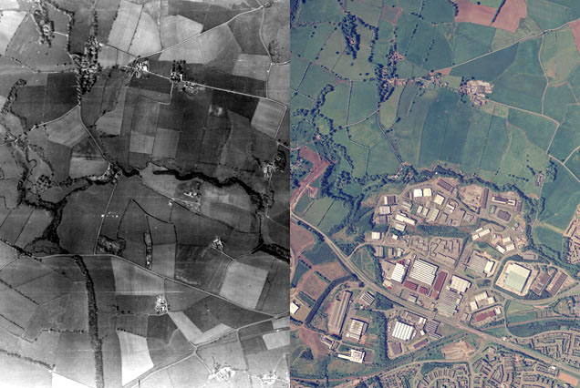
Source: https://ncap.org.uk/sites/default/files/EK_land_use_0.jpg
library(readr)
library(ggplot2)
library(dplyr)
library(caret)
library(rpart.plot)

# Read in the data
land <- read_csv("https://www.macalester.edu/~ajohns24/data/land_cover.csv")

# There are 9 land types, but we'll focus on 3 of them
land <- land %>%
    filter(class %in% c("asphalt", "grass", "tree"))
Exercise 1: Core theme: parametric/nonparametric
What does it mean for a method to be nonparametric? In general, when might we prefer nonparametric to parametric methods? When might we not?
Where do you think trees fall on the parametric/nonparametric spectrum?
Exercise 2: Core theme: Tuning parameters and the BVT
The key feature governing complexity of a tree model is the number of splits used in the tree. How is the number of splits related to model complexity, bias, and variance?
In practice, the number of splits is controlled indirectly through the following tuning parameters. For each, discuss how low/high parameter settings would affect the number of tree splits.
minsplit: the minimum number of observations that must exist in a node in order for a split to be attempted.minbucket: the minimum number of observations in any leaf node.cp: complexity parameter. Any split that does not increase node purity bycpis not attempted.maxdepth: Set the maximum depth of any node of the final tree. The depth of a node is the number of branches that need to be followed to get to a given node from the root node. (The root node has depth 0.)
Exercise 3: Building trees in caret
Fit a tree model for the class outcome (land type), and allow all possible predictors to be considered (~ . in the model formula).
- Use 10-fold CV.
- Choose a final model whose test overall accuracy is within one standard error of the overall best metric.
- The Gini index impurity measure can be a minimum of zero and has an upper bound of 1. Thus, we’ll try a sequence of 50
cpvalues from 0 to 0.5.
Make a plot of test performance versus the cp tuning parameter. Does it look as you expected?
set.seed(___)
tree_mod <- train(

)
Exercise 4: Visualizing trees
Let’s visualize the difference between the trees learned under cp parameters. The code below fits a tree for a lower than optimal cp value (tree_mod_lowcp) and a higher than optimal cp (tree_mod_highcp). We then plot these trees (1st and 3rd) along with our best tree (2nd).
Look at page 3 of the rpart.plot package vignette (an example-heavy manual) to understand what the plot components mean.
tree_mod_lowcp <- train(
    class ~ .,
    data = land,
    method = "rpart",
    tuneGrid = data.frame(cp = 0),
    trControl = trainControl(method = "cv", number = 10),
    metric = "Accuracy",
    na.action = na.omit
)
tree_mod_highcp <- train(
    class ~ .,
    data = land,
    method = "rpart",
    tuneGrid = data.frame(cp = 0.1),
    trControl = trainControl(method = "cv", number = 10),
    metric = "Accuracy",
    na.action = na.omit
)

# Plot all 3 trees in a row
par(mfrow = c(1,3))
rpart.plot(tree_mod_lowcp$finalModel)
rpart.plot(tree_mod$finalModel)
rpart.plot(tree_mod_highcp$finalModel)
Verify for a couple of splits the idea of increasing node purity/homogeneity in tree-building. (How is this idea reflected in the numbers in the plot output?)
Tuning classification trees (like with the
cpparameter) is also referred to as “pruning”. Why does this make sense? NOTE: If “pruning” is a new word to you, first Google it.