Topic 12 Trees (Part 2)

Exercises

You can download a template RMarkdown file to start from here.

Context

Our goal will be to classify types of urban land cover in small subregions within a high resolution aerial image of a land region. Data from the UCI Machine Learning Repository include the observed type of land cover (determined by human eye) and “spectral, size, shape, and texture information” computed from the image. See this page for the data codebook.

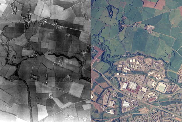
Source: https://ncap.org.uk/sites/default/files/EK_land_use_0.jpg

library(readr)
library(ggplot2)
library(dplyr)
library(caret)
library(rpart.plot)

# Read in the data
land <- read_csv("https://www.macalester.edu/~ajohns24/data/land_cover.csv")

# There are 9 land types, but we'll focus on 3 of them
land <- land %>% 
    filter(class %in% c("asphalt", "grass", "tree"))

Exercise 1: Predictions from trees

Last time, we built a classification tree to predict land type of an image patch (class) from the spectral, size, shape, and texture predictors in the dataset.

Looking at the plot of the fitted tree, manually make a soft (probability) and hard (class) prediction for the case shown below. (See page 3 of the rpart.plot package vignette for a refresher on what the plot shows.)

set.seed(186)
tree_mod <- train(
    class ~ .,
    data = land,
    method = "rpart",
    tuneGrid = data.frame(cp = seq(0, 0.5, length.out = 50)),
    trControl = trainControl(method = "cv", number = 10, selectionFunction = "oneSE"),
    metric = "Accuracy",
    na.action = na.omit
)
rpart.plot(tree_mod$finalModel)

# Pick out training case 2 to make a prediction
test_case <- land[2,]
# Show only the needed predictors
test_case %>% select(NDVI, Bright_100, SD_NIR)

Verify your predictions with the predict() function. (Note: we introduced this code in Logistic Regression, but this type of code applies to any classification model fit in caret).

# Soft (probability) prediction
predict(tree_mod, newdata = test_case, type = "prob")

# Hard (class) prediction
predict(tree_mod, newdata = test_case, type = "raw")

Exercise 2: Reinforcing the BVT

Last time, we looked at a number of different tuning parameters that impact the number of splits in a tree. Let’s focus on minbucket described below.

minbucket: the minimum number of observations in any leaf node.

How would you expect a plot of test accuracy (how is test accuracy estimated again?) vs. minbucket to look, and why? (Draw it!) What part of the plot corresponds to overfitting? To underfitting?
How would you expect a plot of training accuracy vs. minbucket to look, and why? (Draw it!) What part of the plot corresponds to overfitting? To underfitting?

Exercise 3: Variable importance in trees

We can obtain numerical variable importance measures from trees. These measure, roughly, “the total decrease in node impurities from splitting on the variable” (even if the variable isn’t ultimately used in the split).

What are the 3 most important predictors by this measure? Does this agree with you might have expected based on the plot of the fitted tree in Exercise 1? What might greedy behavior have to do with this?

tree_mod$finalModel$variable.importance

Exercise 4: Regression trees

As discussed in the video, trees can also be used for regression! Let’s work through a step of building a regression tree by hand.

For the two possible splits below, determine the better split for the tree by computing the sum of squared residuals as the measure of node impurity. (The numbers following Yes: and No: indicate the outcome value of the cases in the left (Yes) and right (No) regions.)

Split 1: x1 < 3
    - Yes: 1, 1, 2, 4
    - No: 2, 2, 4, 4

Split 2: x1 < 4
    - Yes: 1, 1, 2
    - No: 2, 2, 4, 4, 4

Extra!

In case you want to explore building regression trees in R, try out the following exercises using the College data from the ISLR package. Our goal was to predict graduation rate (Grad.Rate) as a function of other predictors. You can look at the data codebook with ?College in the Console.

library(ISLR)

data(College)

# A little data cleaning
college_clean <- College %>% 
    mutate(school = rownames(College)) %>% 
    filter(Grad.Rate <= 100) # Remove one school with grad rate of 118%
rownames(college_clean) <- NULL # Remove school names as row names

Adapt our general decision tree code for the regression setting by adapting the metric used to pick the final model. (Note how other parts stay the same!)

Note about tuning the cp parameter: rpart uses the R-squared metric to prune branches. (The R-squared metric must increase by cp at each step for a split to be considered.)

set.seed(132)
tree_mod_college <- train(
    Grad.Rate ~ .,
    data = college_clean,
    method = "rpart",
    tuneGrid = data.frame(cp = seq(0, 0.2, length = 50)),
    trControl = trainControl(method = "cv", number = 10, selectionFunction = "oneSE"),
    metric = ___,
    na.action = na.omit
)

Plot test performance as a function of cp, and comment on the shape of the plot.
Plot the “best” tree. (See page 3 of the rpart.plot package vignette for a refresher on what the plot shows.) Do the sequence of splits and outcomes in the leaf nodes make sense?
Look at the variable importance metrics from the best tree. Do the most important variables align with your intuition?