Topic 3 Accuracy Metrics for Regression

3.1 Discussion

Evaluating regression models

Should meet assumptions required for statistical inference
Should explain a substantial proportion of the variation in the response
Should produce accurate predictions

For both of these points, we can look at residuals.

Sum of squared residuals

\[RSS = \sum_{i=1}^n (y_i - \hat{y_i})^2 = (y_1 - \hat{y}_1)^2 + (y_2 - \hat{y}_2)^2 + \cdots + (y_n - \hat{y}_n)^2\]

The sum (and mean) of the residuals is always zero when an intercept is included in the linear regression model -> add up the squared residuals
Not very interpretable
Due to missing values in predictors, sample size can vary from analysis to analysis (hard to compare RSS)

Mean squared error

\[MSE = \frac{RSS}{n} = \frac{1}{n}\sum_{i=1}^n (y_i - \hat{y}_i)^2\]

More interpretable than RSS: on average how far are our predictions from the true values (in squared distance)?
Interpretation downside: the units are squared units
Square root of MSE (RMSE = root mean squared error) is often used:
\(RMSE = \sqrt{MSE}\)
It’s tempting to try to interpret RMSE as the average distance of our predictions from the true values because the units align with the response variable, but it’s not technically quite right due to the square root.

Mean absolute error

\[MAE = \frac{1}{n}\sum_{i=1}^n \|y_i - \hat{y}_i\|\]

Where \(\|y_i - \hat{y}_i\|\) indicates the absolute value of the residual

Very interpretable: on average how far are our predictions from the true values

R-squared

Define the total sum of squares (\(TSS\)) as the sum of squared deviations of each response \(y_i\) from the mean response \(\bar{y}\):

\[TSS = \sum_{i=1}^n (y_i - \bar{y})^2\]

\[R^2 = 1-\frac{RSS}{TSS} = \frac{\text{Var(fitted)}}{\text{Var(response)}}\]

Very interpretable: the proportion of variation in the response that is explained by the model

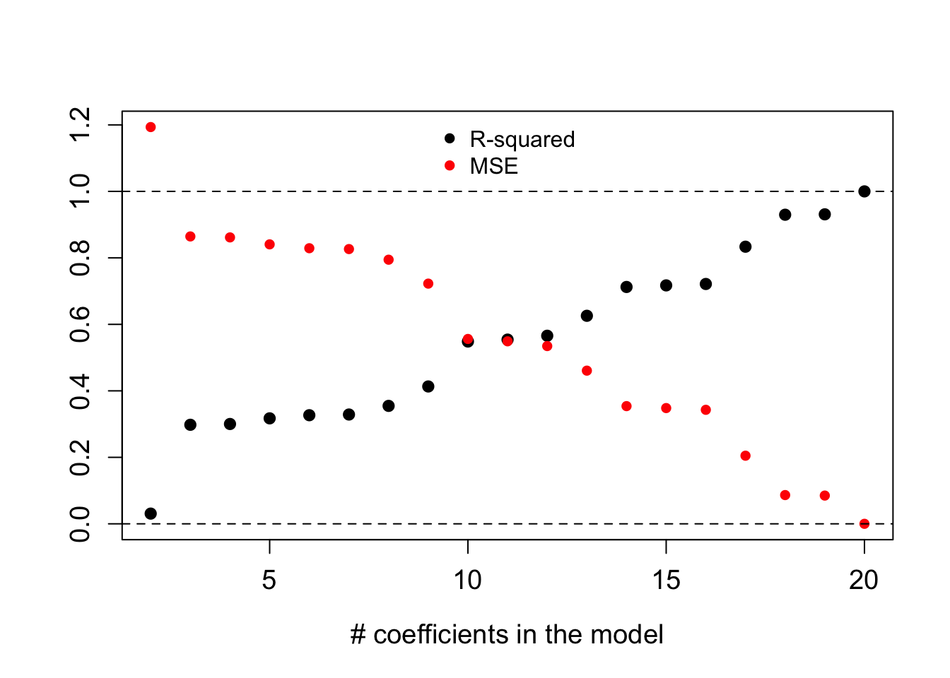
Problems with R-squared and MSE

R-squared automatically increases with added predictors (even useless ones)
MSE automatically decreases with added predictors (even useless ones)
Example below: dataset with 20 cases. Random numbers are used as predictors.

Alternative metrics:
- Instead of R-squared, use adjusted R-squared
- Instead of MSE, we’ll use cross-validation (coming up next)

Overfitting

The example above is a demonstration of overfitting.
With more and more predictors, greater chance that some are useless.
Including useless predictors in a model is like reading too much into the noise.
With overfitting, models don’t tend to generalize well.

3.2 Exercises

You can download a template RMarkdown file to start from here.

You’ll be working a dataset containing physical measurements on 80 adult males. These measurements include body fat percentage estimates as well as body circumference measurements.

fatBrozek: Percent body fat using Brozek’s equation: 457/Density - 414.2
fatSiri: Percent body fat using Siri’s equation: 495/Density - 450
density: Density determined from underwater weighing (gm/cm^3).
age: Age (years)
weight: Weight (lbs)
height: Height (inches)
neck: Neck circumference (cm)
chest: Chest circumference (cm)
abdomen: Abdomen circumference (cm)
hip: Hip circumference (cm)
thigh: Thigh circumference (cm)
knee: Knee circumference (cm)
ankle: Ankle circumference (cm)
biceps: Biceps (extended) circumference (cm)
forearm: Forearm circumference (cm)
wrist: Wrist circumference (cm)

It takes a lot of effort to estimate body fat percentage accurately through underwater weighing. The goal is to build the best predictive model for fatSiri using just circumference measurements, which are more easily attainable. (Don’t use fatBrozek or density as predictors.)

library(ggplot2)
library(dplyr)
bodyfat <- read.csv("https://www.dropbox.com/s/js2gxnazybokbzh/bodyfat_train.csv?dl=1")

# Remove the fatBrozek and density variables
bodyfat <- bodyfat %>%
    select(-fatBrozek, -density)

Using tools from Math 155 and 253 (e.g. exploratory plots, p-values, confidence intervals, adjusted R-squared), experiment with different models to try to build the best predictive model possible. What are the adjusted R-squared and MSE for this model?

Code notes: if you want to extract the adjusted R-squared from a fitted model, you can use the following.

your_model <- lm(fatSiri ~ age, data = bodyfat)
summary(your_model)$adj.r.squared

And if you want to compute MSE, you can use the function below:

mse <- function(mod) {
    mean(residuals(mod)^2)
}
mse(your_model)

Now that you’ve selected your best model, deploy it in the real world by applying it to a new set of 172 adult males. The predict() function allows you to supply a fitted model and a new dataset of predictors (the newdata argument).

bodyfat_test <- read.csv("https://www.dropbox.com/s/7gizws208u0oywq/bodyfat_test.csv?dl=1")

# Predict
test_predictions <- predict(your_model, newdata = bodyfat_test)

# Compute MSE
# The $ extracts a particular column from a dataset
mean((bodyfat_test$fatSiri - test_predictions)^2)

Thinking about main themes
1. How did your MSE on the original dataset of 80 males compare to the MSE on the new data of 172 males?
2. What conclusions can you draw from this exploration in relation to overfitting?

Thinking more about overfitting
1. Do you think that a model with more predictors or less predictors is more prone to overfitting? Why?
2. The method used to find the coefficients in linear regression is called the least squares method. We find coefficients \(\hat{\beta}_1, \hat{\beta}_2, \ldots, \hat{\beta}_p\) that minimize the sum of squared residuals \(RSS\). Given your answer in part a, can you think of a way to modify the least squares criterion to penalize weak predictors being included in a model? That is, can you brainstorm a possible penalty to add below?
  Least squares criterion: find \(\hat{\beta}_1, \ldots, \hat{\beta}_p\) that minimize \(RSS\)
  Penalized least squares criterion: find \(\hat{\beta}_1, \ldots, \hat{\beta}_p\) that minimize \(RSS + \text{penalty}\)
  Suggestion: Draw inspiration from the “penalty” term in the adjusted R-squared formula from the video.

Extra! If you have time and are interested in learning about writing R functions, try the following.
1. Using the mse() function above as a guide, write a function that compute the MSE of a model on new data.
  - What inputs do you need? These must be supplied as arguments to the function. These are given in the parentheses.
  - You can take multiple intermediate steps within the function. This is often recommended for multi-step tasks because it makes the code easier to read.
  - Annotate the steps of your function with comments. (Start a comment line with a #.)