Topic 12 Decision Trees

12.1 Discussion

Why trees?

Logistic regression is a parametric method.
- Also can only model binary responses
If we don’t think that the model form below holds, might prefer a nonparametric method \[\text{log odds} = \beta_0 + \beta_1 x_1 + \cdots + \beta_p x_p\]
Nonparametric methods
- KNN classification
- Tree-based methods
Both KNN and tree-based methods can handle 3+ classes.

Gini index: choosing the “best” binary split

Suppose:

response variable $y$ has $C$ different classes
the tree has $R$ total regions/nodes (leaves)

Measuring the purity of a single node

Let

\[p_{rc} = \text{proportion of cases in region/node $r$ that are of class $c$}\]

From these, we can compute the node/region’s Gini index/impurity:

\[G_r = \sum_{c=1}^C p_{rc} (1 - p_{rc})\]

The smaller $G_r$, the more pure region $r$ is.
$G_r = 0$ if region $r$ is perfectly pure (the cases in the node are all of 1 class).

Choosing the binary splits

The binary splits in a tree are chosen to minimize the average Gini index across all regions:

\[\sum_{r=1}^{R} G_r \cdot \frac{\text{# cases in region r}}{\text{total # cases}}\]

Example

13 cases; 3 classes (A, B, and C)

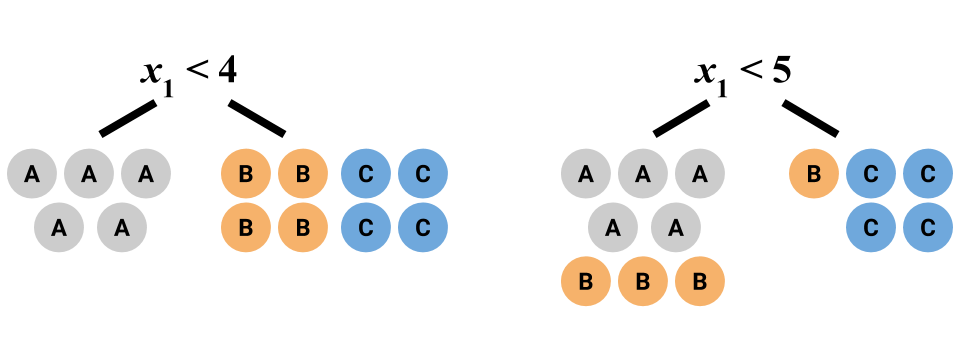
What is the average Gini index for the first split? For the second split? Which split is preferable?

12.2 Exercises

You can download a template RMarkdown file to start from here.

Why use the Gini index instead of classification accuracy to build the tree? Consider a situation where we have 2 classes (class A and B) with 400 cases in each class. Consider two different splits:
Split 1:
Node 1 has 300 cases of class A and 100 of class B
Node 2 has 100 cases of class A and 300 of class B
Split 2:
Node 1 has 200 cases of class A and 400 of class B
Node 2 has 200 cases of class A and 0 of class B
1. To make a prediction for a node, we predict the majority class for all cases in that node. (e.g. For Split 1, Node 1, we predict A for all cases in that node.) What is the overall accuracy over both Nodes 1 and 2 for Split 1? For Split 2?
2. What is the average Gini index for Split 1? For Split 2?
3. Based on this example, why do you think the Gini index is preferred?

Trees can also be used for regression!
For classification, we use average Gini index as a measure of node (im)purity for tree building. We can build regression trees using residuals. In particular, we try to find the particular predictor and split point that minimize the following equation: \[\sum_{i: x_i \in R_1} (y_i - \hat{y}_{R_1})^2 + \sum_{i: x_i \in R_2} (y_i - \hat{y}_{R_2})^2\] There’s a lot of notation in the above equation, but we can break it down into two sensible pieces. $\hat{y}_{R_1}$ and $\hat{y}_{R_2}$ are the predicted values in region(/node/leaf) 1 and region 2. (Regions 1 and 2 are the left and right branches.) These predicted values are the mean of the cases that end up in that region. The left sum is the sum of squared residuals in region 1, and the right sum is the sum of squared residuals in region 2.
Explain why minimizing the above equation is sensible for building regression trees.

Those greedy, greedy algorithms…
It was mentioned in the video that recursive binary splitting (RBS) is a greedy algorithm. What is another technique we’ve learned in class that is greedy? Describe how RBS parallels that other technique.

Overfitting and the bias-variance tradeoff
Consider the two trees below built from a heart disease dataset.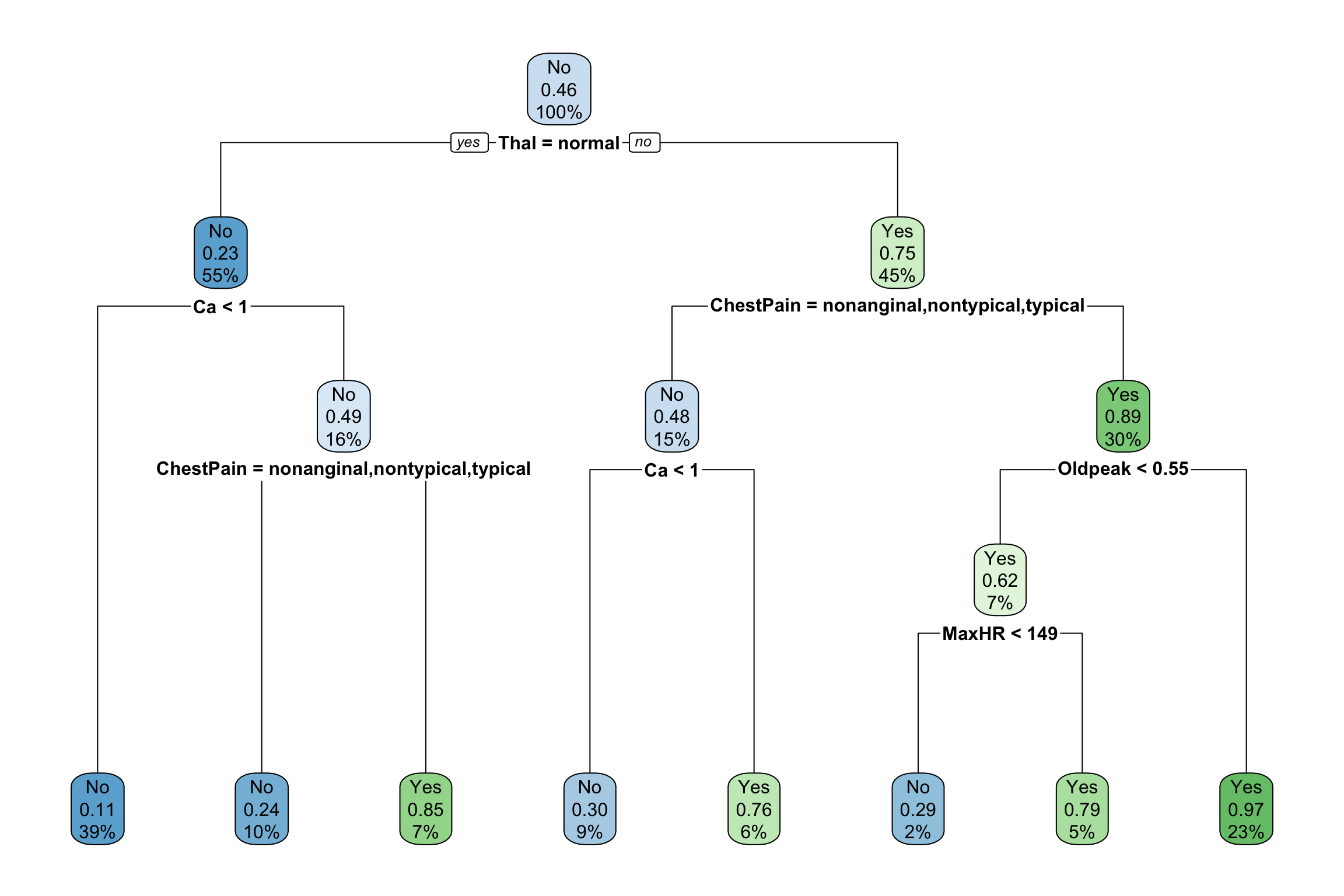
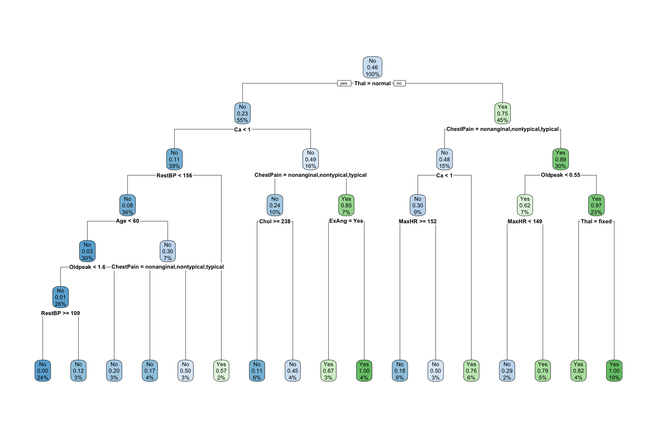
1. Which tree is likely overfit to the data and why?
2. Number of splits is not something that we can often directly control when we use software to build decision trees, but we can still think of it as a tuning parameter. How is number of splits related to bias and variance?

Tree pruning
The idea behind tree pruning is to first grow a large tree. (e.g. Grow each region until the leaves have 5 or fewer cases.) Then we prune some branches–that is, we take out some splits. If there was a split, merge it back together.
1. The big tree above was actually pruned to make the smaller tree. Compare the trees and verify for a couple of branches that the changes result from merging nodes back together.
2. This pruning is achieved with something called cost complexity pruning, and the idea is very related to LASSO! The cost complexity criterion for classification trees looks like: \[\text{average Gini index over leaves} + \alpha \times (\text{# leaves})\] Describe how this pruning criterion helps with overfitting by discussing the 2 extremes of $\alpha$. How can we pick a good value for $\alpha$?

In the exercises below, we’ll work with some real data and caret to nail down some computing essentials for decision trees.

You’ll be looking at high resolution aerial image data to classify different parts of images into different types of urban land cover. Data from the UCI Machine Learning Repository include the observed type of land cover (determined by human visual inspection) and “spectral, size, shape, and texture information” computed from the image.

There are 9 types of land uses in the dataset. We’ll focus on distinguishing between asphalt, grass, and tree.

library(ggplot2)
library(dplyr)

land <- read.csv("https://www.macalester.edu/~ajohns24/data/land_cover.csv")
land <- land %>% 
    filter(class %in% c("asphalt ","grass ", "tree ")) %>% 
    mutate(class = droplevels(class))

Before moving forward, install the rpart and rpart.plot packages in the Console. rpart builds decision trees and rpart.plot makes beautiful tree plots.

install.packages(c("rpart", "rpart.plot"))

There are 147 possible predictors of land use class. We can fit a decision tree using all 147 predictors with the code below. 10-fold CV is used to estimate test accuracy. The tuneLength = 30 means that 30 values of the tree’s tuning parameter are tried. This tuning parameter is called the cp or “Complexity Parameter” and can be viewed similarly to $\alpha$ in Exercise 5. That is, high values of this parameter are akin to high values of $\alpha$.
```
library(caret)
library(rpart)
library(rpart.plot)

set.seed(333)
tree_mod1 <- train(
    class ~ .,
    data = land,
    method = "rpart",
    metric = "Accuracy",
    trControl = trainControl(method = "cv", number = 10),
    tuneLength = 30
)
```
1. Plot test accuracy versus this Complexity Parameter. Roughly, what is the optimal value of this parameter?
```
plot(tree_mod1)
```
2. Why does the plot look this way? Specifically, write an explanation that discusses the far left of the plot, the middle, and the far right. Discuss tree complexity, bias, and variance in these 3 parts of the plot.
3. Report the exact value for this optimal value with tree_mod1$bestTune, and report the estimated test accuracy of this tree by looking at tree_mod1$results.
4. Plot the best tree with:
```
rpart.plot(tree_mod1$finalModel)
```
  Look at page 3 of the rpart.plot package vignette (an example-heavy manual) to understand what the plot components mean.
5. What percent of the cases get split into the region defined by the following condition? NDVI >= -0.01, Bright_100 < 142
6. What would be your hard prediction of land use class when NDVI = -0.05?
7. What are the soft predictions of a region being asphalt, grass, tree when NDVI = -0.05? Describe a situation in which these soft predictions would be useful.

There are more tuning parameters than just the cp Complexity Parameter. You can view many ways to control the building of a tree (essentially encoding the stopping criteria) by looking at the help page for the rpart.control() function by entering ?rpart.control in the Console. We will explore the minbucket parameter in this exercise.
1. Read about the minbucket parameter on the help page. What will happen to the number of splits in the tree as minbucket increases?
2. The code below fits a decision tree using the best cp value identified from cross-validation earlier and uses a minbucket of 7 (the default value). Write a for-loop to plot trees for several minbucket values to check your response in part a. Use values from 10 to 70 counting up by 10.
  Hint 1: First create the minbucket sequence using the seq() function.
  Hint 2: You don’t need to create any “empty boxes” to store output because the goal is to just print the trees.
  Hint 3: The inside of the for-loop will be almost identical to what is already below.
```
tree_mod2 <- rpart(
    class ~ .,
    data = land,
    minbucket = 7,
    cp = tree_mod1$bestTune$cp
)
rpart.plot(tree_mod2)
```