Topic 16 K-Means Clustering

16.1 Discussion

Applications of clustering

Biology: Are there species, subspecies of these organisms based on their gene expression, physical measurements?
Chemistry: Are there different groups of compounds? Perhaps based on shape, toxicity to humans?
Sports: Are there different type of players? Based on skill, play style, body type?
Market analysis and economics: Are there certain type of consumers? Purchasing behaviors?
Geography: Are there certain types of neighborhoods?

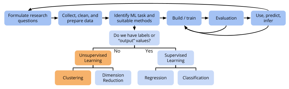
Clustering seems like classification, but is different

In classification, the response variables are used in training the model. The response variables supervise how the model is fit.
In clustering, there might not be a response variable, and we don’t need to use it even if there is. e.g. In the iris dataset, there is a column indicating the flower species, but nothing dictates that the species level (as opposed to subspecies) should be our scientific interest.

Considerations in picking the number of clusters/evaluating clusters

Context!
Also plots of number of clusters versus total within-cluster sums of squares
The combination of the two helps inform the number of groupings that are reasonable for the observed data
Evaluating clustering is hard!
- It’s a joke (but kind of true) that with enough tweaking of clustering parameters, distance metrics, scaling…you could get any clustering that you desired.
- We need to look at multiple variations of the clustering: different methods, parameters.
- What makes sense? e.g. Both 3 clusters and 4 clusters might make sense on different levels. Perhaps you discover that 3 clusters roughly corresponds to level of binge-purchasing behavior and that 4 clusters roughly corresponds to purchasing aligning with 4 distinct categories of hobbies.

Prediction with clustering

Once you have a set of clusters, it’s possible to assign new cases to the closest cluster.
You might find after enough new cases that new clusters might be needed. Re-cluster the data. How do things change? What new insights are gained?

Clustering predictors as opposed to cases

When we cluster cases, we look at distances between cases (distances between rows of our dataset).
When we cluster predictors, we look at distances between predictors (distances between columns of our dataset).
- So clustering predictors involves transposing our dataset.
- PCA is another way to “cluster” predictors. Coming up next!

16.2 Exercises

You can download a template RMarkdown file to start from here.

NOTE: completing these exercises is a part of your Homework 7, due Wednesday, April 10 at midnight.

To iron out the K-means algorithm, we’ll look at a small example of physical measurements (sepal length and width) of 5 irises in the first exercise:

irises <- data.frame(
    Width = c(0.5,0.5,2.3,2.8,3.0),
    Length = c(2.0,2.5,1.3,1.8,1.3)
)
ggplot(irises, aes(x = Width, y = Length)) + 
    geom_point() + 
    geom_text(aes(label = c(1:5)), vjust = 1.5) + 
    lims(x = c(0,4), y = c(0,4))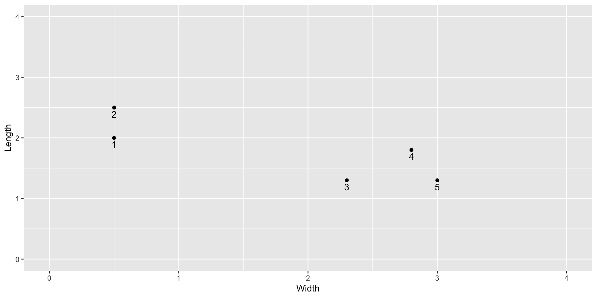

Cluster these 5 flowers by hand using K=2 clusters. For the first stage of initialization, use the random cluster assignments shown below in the cluster column. Show your work for 2 iterations of the centroiding and reassignment steps.

cbind(irises, data.frame(cluster = c(2,1,1,1,2)))

##   Width Length cluster
## 1   0.5    2.0       2
## 2   0.5    2.5       1
## 3   2.3    1.3       1
## 4   2.8    1.8       1
## 5   3.0    1.3       2

You may find it helpful to use this function to calculate the distance of each case to a specified point:

dist_iris <- function(point) {
    sqrt((irises$Width - point[1])^2 + (irises$Length - point[2])^2)
}
# For example: distance of every case to (1,2)
dist_iris(point = c(1,2))

The kmeans() function in R performs K-means clustering. Check your work from the previous exercise.

irises_clust2 <- kmeans(irises, centers = 2)

# Check out the cluster assignments
irises_clust2$cluster

# Plot the clusters
irises <- irises %>% 
    mutate(cluster = irises_clust2$cluster)
ggplot(irises, aes(y = Length, x = Width, color = as.factor(cluster))) + 
    geom_point() + 
    lims(x = c(0,4), y = c(0,4))

In the remainder of the exercises, we’ll look at the full iris dataset of 150 flowers.

data(iris)

Part of performing K-means clustering is choosing an appropriate value for K.
1. To explore the impact of K, perform a K-means cluster analysis of the iris data using just Sepal.Length and Sepal.Width (for ease of visualization). Use the following code for $K=2$ and adapt it to explore $K=3$ and $K=20$.
```
# Take only Sepal.Length & Sepal.Width
iris_sub <- iris %>%
    dplyr::select(Sepal.Length, Sepal.Width)

# K=2 clusters
km_clust2 <- kmeans(iris_sub, centers = 2)
ggplot(iris_sub, aes(x = Sepal.Width, y = Sepal.Length, color = as.factor(km_clust2$cluster))) + 
    geom_point()
```
2. Based on these plots, discuss the pros and cons of low and high K.

Before moving on, let’s get more comfortable working with unfamiliar objects in R.
1. Look at the help page for the kmeans() function and scroll down to the “Value:” section. What is the name of the component of a kmeans object that contains a measure of total within-cluster variation?
2. Whenever we want to extract a certain component of an R object that is a list, we can use the code list_object$name_of_component. Display the measure of total within-cluster variation for km_clust2.

A strategy for picking K is to compare the total squared distance of each case from its assigned centroid (the total within-cluster sum of squares) for different values of K.
1. Write a for-loop to calculate the total sum of squared distances for each K in $\{1, 2, ..., 50\}$. Plot these squared distances versus K.
```
# Create storage vector for total within-cluster sum of squares
tot_wc_ss <- rep(0, 50)

# Loop
for (i in 1:50) {
    # Perform k means clustering on iris_sub
    ???

    # Store the total within-cluster sum of squares
    tot_wc_ss[i] <- ???$???
}
plot(1:50, tot_wc_ss)
```
2. Based on this plot, which values of K seem reasonable? Explain.

Extra! Think about the scientific questions that you want to answer for your final project. Could clustering play a role in your scientific pursuits?