B Splines
Disclaimer: These exercises are by no means required or knowledge that I expect you to be responsible for. But if you want to dig deeper into the math of splines, try these out.
Background: A cubic spline is a function that consists of piecewise polynomials stitched together continuously over multiple regions. The spline must also have continuous first and second derivatives at the knots. The exercise below draws from Exercise 1 in Chapter 7 of ISLR. Through it, you’ll see how a spline function can be modeled via linear regression by transforming the predictor variable multiple times.
B.1 Exercise
We’ll be in a situation where there is one knot at \(x = k\). Consider the function
\[f(x) = \beta_0 + \beta_1x + \beta_2 x^2 + \beta_3 x^3 + \beta_4 (x-k)^3_+\]
where the + in \((x-k)^3_+\) denotes the positive part. That is, \((x-k)^3_+\) equals \((x-k)^3\) when \(x > k\) and equals 0 otherwise.
Overall goal: Show that a function of the form above is a cubic spline. That is, we must show that:
- \(f(x)\) consists of two piecewise cubic polynomials: \(f_1(x)\) in region 1 where \(x \leq k\) and \(f_2(x)\) in region 2 where \(x > k\)
- \(f(x)\) is continuous at \(x = k\)
- The first derivative \(f'(x)\) is continuous at \(x = k\)
- The second derivative \(f''(x)\) is continuous at \(x = k\)
Goal 1: Show that \(f(x)\) consists of two piecewise cubic polynomials.
- Show that in region 1, we can write the region-specific polynomial as a cubic. That is, \(f_1(x)\) should look like \(f_1(x) = a_1 + b_1x + c_1x^2 + d_1x^3\) for some values of \(a_1, b_1, c_1, d_1\) related to \(\beta_0, \beta_1, \beta_2, \beta_3, \beta_4\) and possibly also \(k\).
- Show that in region 2, we can write the region-specific polynomial as a cubic. That is, \(f_2(x)\) should look like \(f_2(x) = a_2 + b_2x + c_2x^2 + d_2x^3\) for some values of \(a_2, b_2, c_2, d_2\) related to \(\beta_0, \beta_1, \beta_2, \beta_3, \beta_4\) and possibly also \(k\).
Goal 2: Show that \(f(x)\) is continuous at \(x = k\).
Goal 3: Show that \(f'(x)\) is continuous at \(x = k\).
Goal 4: Show that \(f''(x)\) is continuous at \(x = k\).
B.2 Debriefing
Great! Now that we’ve shown that the function above gives the general form of a spline, we see that we go back to a least squares linear regression framework. Our response \(y\) is modeled as
\[y = f(x) + \varepsilon\]
We see from the form of \(f(x)\) that modeling \(y\) as a nonlinear function of \(x\) just involves “spline-ifying” \(x\). We do that by transforming \(x\) 4 times:
- \(x\) raised to the power 1 (associated with coefficient \(\beta_1\))
- \(x\) raised to the power 2 (associated with coefficient \(\beta_2\))
- \(x\) raised to the power 3 (associated with coefficient \(\beta_3\))
- \(x\) minus the knot location \(k\), raised to the power 3, and finally take the positive part (associated with coefficient \(\beta_4\))
Note: The 4 transformation functions that we’ve looked at here are 4 possible ones. A drawback you may notice is that if \(x\) is large, using these transformations involves cubing large numbers, which can be numerically unstable.
There are other sets of 4 transformations that can be combined as above to make \(f(x)\) a cubic spline overall. (In linear algebra terms, there are other bases of functions that still span the vector space of piecewise polynomials that are continuous and have continuous first and second derivatives at the knots. What has been represented above is a linear combination of basis functions.) In particular, when you use functions like ns() in R, R uses a different set of transformation functions, which are the colored functions like below plotted in the video and in the course manual.
library(splines)
set.seed(57)
n <- 1000
x <- seq(0, 2*pi, length.out = n)
y <- sin(x) + rnorm(n, mean = 0, sd = 0.5)
spline_terms_df2 <- ns(x, df = 2)
spline_terms_df4 <- ns(x, df = 4)
spline_terms_df8 <- ns(x, df = 8)
par(mfrow = c(1,4))
plot(x, y, main = "y = sin(x)")
matplot(spline_terms_df2, type = "l", xlab = "x", ylab = "Transformed x", main = "df = 2")
matplot(spline_terms_df4, type = "l", xlab = "x", ylab = "Transformed x", main = "df = 4")
matplot(spline_terms_df8, type = "l", xlab = "x", ylab = "Transformed x", main = "df = 8")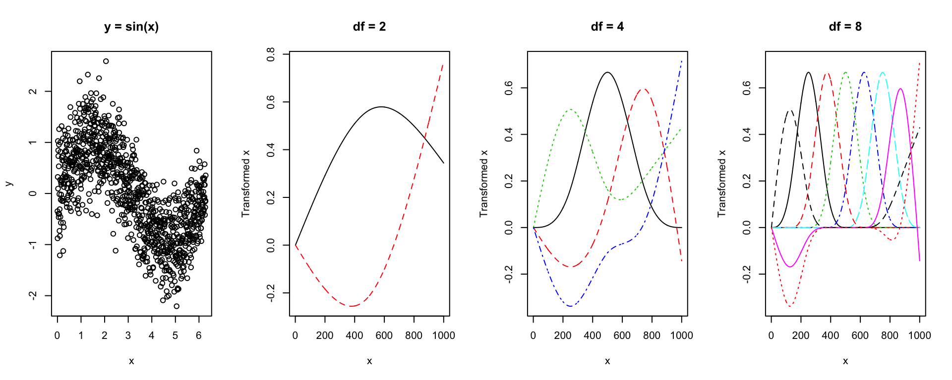
The details of the particular algorithm that R uses involves a lot of tedious recursive formulas, which, frankly, the instructor finds confusing and completely unilluminating, which is why we won’t go down that path. If you are interested in looking at this, search for “B-spline algorithm” (B-spline stands for “basis spline”).